étude de l'efficience des marchés financiers. Cas de DZAIR index.

Annexes

Cours de société :ALLIANCE

Colonne1 2016-04-04	Colonne2 505	dividende	Colonne4 -1.94%
2016-05-02	500		-0.99%
2016-06-01	500	35	7.00%
2016-07-04	475		-5.00%
2016-08-01	465		-2.11%
2016-09-05	465		0.00%
2016-10-04	465		0.00%
2016-11-03	470		1.08%
2016-12-05	465		-1.06%
2017-01-02	465		0.00%
2017-02-01	465		0.00%
2017-03-01	465		0.00%
2017-04-03	450		-3.23%
2017-05-02	445		-1.11%
2017-06-05	445	45	10.11%
2017-07-03	400		-10.11%
2017-08-02	420		5.00%
2017-09-04	420		0.00%
2017-10-02	420		0.00%
2017-11-02	420		0.00%
2017-12-04	420		0.00%
2018-01-02	420		0.00%
2018-02-05	420		0.00%
2018-03-05	420		0.00%
2018-04-02	425		1.19%
2018-05-03	425		0.00%
2018-06-04	430		1.18%
2018-07-02	430	45	10.47%
2018-08-01	395		-8.14%
2018-09-03	410		3.80%
2018-10-02	420		2.44%
2018-11-04	420		0.00%
2018-12-02	426		1.43%
2019-01-02	427		0.23%
2019-02-03	429		0.47%
2019-03-03	449		4.66%
2019-04-02	431		-4.01%
rendement			0.08%
variance			0.17%
ecart type			4.14%

103

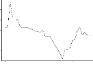
En utilisant les instruction de R : Les cours:

>rouiba=c(365,375,375,375,370,360,380,380,375,370,360,355,355,345,315,315,300,390,370,370,350,350,335,3

35,335,330,325,325,325,325,325,325,320,300,300,300,300,300,300,300,295,295,295,295,295,295,295,266,266, 240,240,235)

>time_series=ts(rouiba,start = 2015,end = 2019,frequency=12) >plot(time_series)

>time_series = ts(biopharm, start=2016,end=2019,frequency=12) >plot(time_series , main= `biopharm `,xlab= `year', ylab='cours')

^biopharm

^{2016 2017 2018 2019}

^Time

Test de dickey-fuller surdzindex : >library(urca)

>r=diff(log(dzindex))

>x=ur.df(r,type='trend',lag=1);summary(x)

############################################### # Augmented Dickey-Fuller Test Unit Root Test #

###############################################

Test regression trend

Call:

lm(formula = z.diff ~ z.lag.1 + 1 + tt + z.diff.lag)

Residuals:

Min 1Q Median 3Q Max

-0.068868 -0.019320 -0.004815 0.010043 0.136536

Coefficients:

Estimate Std. Error t value Pr(>|t|)

(Intercept) 2.449e-03	9.864e-03	0.248 0.805
z.lag.1 -9.712e-01	2.107e-01	-4.610 3.21e-05 ***
tt 4.274e-05	3.272e-04	0.131 0.897
z.diff.lag -5.160e-02	1.466e-01	-0.352 0.726
Signif. codes: 0 `***'	0.001 `**'	0.01 `*' 0.05 `.' 0.1	`	'	1

Residual standard error: 0.03334 on 46 degrees of freedom

Multiple R-squared: 0.515, Adjusted R-squared: 0.4834

104

F-statistic: 16.28 on 3 and 46 DF, p-value: 2.381e-07 Value of test-statistic is: -4.6102 7.0895 10.6341

Critical values for test statistics: 1pct 5pct 10pct
tau3	-4.04 -3.45		-3.15
phi2	6.50	4.88	4.16
phi3	8.73	6.49	5.47

Test de dickey-fuller sur ROUIBA :

>rouiba=c(365,375,375,375,370,360,380,380,375,370,360,355,355,345,315,315,3 00,390,370,370,350,350,335,335,335,330,325,325,325,325,325,325,320,300,300, 300,300,300,300,300,295,295,295,295,295,295,295,266,266,240,240,235) >r=diff(log(rouiba))

>x=ur.df(r,type='trend',lag=1);summary(x)

############################################### # Augmented Dickey-Fuller Test Unit Root Test #

###############################################

Test regression trend

Call:

lm(formula = z.diff ~ z.lag.1 + 1 + tt + z.diff.lag)

Residuals:

Min 1Q Median 3Q Max

-0.092416 -0.015044 -0.000449 0.015047 0.257674

Coefficients:

Estimate Std. Error t value Pr(>|t|)

(Intercept) 0.0006850	0.0145024	0.047 0.963
z.lag.1 -1.1186352	0.2343856	-4.773 1.95e-05 ***
tt -0.0004370	0.0005008	-0.873 0.387
z.diff.lag -0.1067734	0.1480586	-0.721 0.475
Signif. codes: 0 `***'	0.001 `**'	0.01 `*' 0.05 `.' 0.1	`	'	1

Residual standard error: 0.04844 on 45 degrees of freedom Multiple R-squared: 0.6304, Adjusted R-squared: 0.6058 F-statistic: 25.59 on 3 and 45 DF, p-value: 8.206e-10

Value of test-statistic is: -4.7726 7.6036 11.3987

Critical values for test statistics: 1pct 5pct 10pct
tau3	-4.04 -3.45		-3.15
phi2	6.50	4.88	4.16
phi3	8.73	6.49	5.47

Test de dickey-fuller sur SAIDAL:

>SAIDAL=c(560,560,560,560,570,575,585,605,580,635,640,660,640,640,640,635,6

40,640,640,640,600,600,600,600,600,600,640,635,665,665,665,665,660,660,660,

660,660,640,620,620,620,620,620,580,580,605,605,635,635,635,610,609)

r=diff(log(SAI))

>x=ur.df(r,type='trend',lag=1);summary(x)

############################################### # Augmented Dickey-Fuller Test Unit Root Test #

105

############################################### Test regression trend

Call:

lm(formula = z.diff ~ z.lag.1 + 1 + tt + z.diff.lag)

Residuals:

Min 1Q Median 3Q Max

-0.068347 -0.007393 -0.000309 0.007837 0.072081

Coefficients:

Estimate Std. Error t value Pr(>|t|)

(Intercept) 0.0100816	0.0084123	1.198 0.237019
z.lag.1 -0.9566756	0.2242311	-4.266 0.000101 ***
tt -0.0003302	0.0002823	-1.170 0.248285
z.diff.lag -0.1701993	0.1493245	-1.140 0.260402
Signif. codes: 0 `***'	0.001 `**'	0.01 `*' 0.05 `.' 0.1	`	'	1

Residual standard error: 0.02734 on 45 degrees of freedom Multiple R-squared: 0.5882, Adjusted R-squared: 0.5607 F-statistic: 21.42 on 3 and 45 DF, p-value: 9.084e-09

Value of test-statistic is: -4.2665 6.1067 9.1494

Critical values for test statistics: 1pct 5pct 10pct
tau3	-4.04 -3.45		-3.15
phi2	6.50	4.88	4.16
phi3	8.73	6.49	5.47

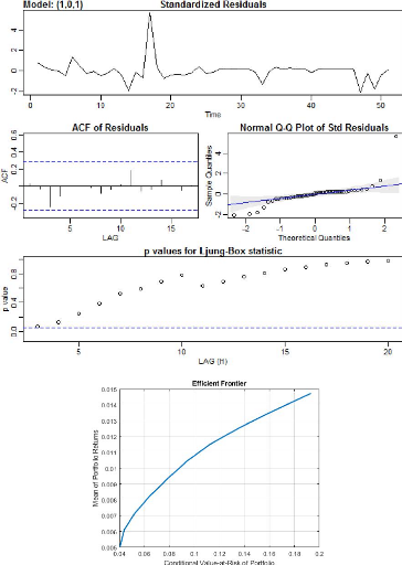
prevision de la serie NC-ROUIBA

>sarima.for(r,n.ahead=12,p=1,d=0,q=1)

$pred

Time Series:

Start = 52

End = 63

Frequency = 1
[1]	0.003725608	-0.018144936	-0.001074932	-0.014398105	-0.003999341
[6]	-0.012115598	-0.005780842	-0.010725132	-0.006866104	-0.009878083		[11]
-0.007527227	-0.009362075

$se

Time Series: Start = 52 End = 63

Frequency = 1								[1]
0.04563118	0.04648744	0.04700142	0.04731179	0.04749987	0.04761408		[7]
0.04768352	0.04772577	0.04775150	0.04776716	0.04777670	0.04778251

>library(quantmod) >getSymbols("AMZN", from = "2000-01-01", to = "2019-01-01", src = "yahoo",

adjust = TRUE)

106

GOOGLE >getSymbols("GOOG", from = "1980-12-01", to = "2018-12-31", src = "yahoo",

adjust = TRUE) >plot(Cl(GOOG))

FACEBOOK

1 ) Importer les données : >Library (quantmod) >getSymbols("FB", from = "2012-05-01", to = "2018-12-31", src = "yahoo",

>plot(Cl(FB))

107

NC4-ROUIRAI
SPA

ETATS FINANCIERS 31.12.2918

~a

COMPTE DE RESULTATS PERIODE DU 01.01.2018 AU 31.12.2018
CHIFFRES EXPRIMES EN DINARS

	NOTE		31.12.2018					31.12.2017
Chiffre d'affaires	6.1		5 936 615 369					5 659 391 237
Variation stocks produits finis et en-cours	6.2		( 164 687 788)					260 096 158
Production immobilisée
Subventions d'exploitation
PRODUCTION DE L'EXERCICE			5 771 927 581					5 919 487 396
Achats consommés	6.3		(3 618 612 603)					(3 607 011 260)
Services extérieurs et autres consommations	6.4		( 926 986 537)					(1 129 603 933)
CONSOMMATION DE L'EXERCICE			(4 545 599 140)					(4 736 615 193)
VALEUR AJOUTEE D'EXPLOITATION			1 226 328 441					1 182 872 203
Charges de personnel	6.5		( 711 630 826)					( 722 931 844)
Impôts taxes et versements assimilés	6.6		(50 733 316)					(54 753 822)
EXCEDENT BRUT D'EXPLOITATION			463 964 299					405 186 536
Autres produits opérationnels	6.7		89 892 128					47 099 948
Autres charges opérationnelles	6.8		( 127 735 114)					( 138 477 963)
Dotations aux amortissements et aux provisions	6.9		(534682928)					(744037721)
Reprise sur pertes de valeur et provisions			49 028 820					3 247 456
RESULTAT OPERATIONNEL			( 59 532 796)					( 426 981 745)
Produits financiers	6.10		21 728 182					15 082 804
Charges financières	6.11		( 290 470 023)					( 375 831 347)
RESULTAT FINANCER			( 268 741 841)					( 360 748 543)
RESULTAT ORDINAIRE AVANT IMPÔTS			( 328 274 637)					( 787 730 288)
Impôts exigibles sur résultat ordinaires Impôts différés sur résultats ordinaires Total des produits des activistes ordinaires		5		985	53 238 671 815 381		6		070	85 120 037 037 641
Total des charges des activités ordinaires		(6		260	851	347)	(6		772	647	891)
RESULTAT NET DES ACTIVITES ORDINAIRES		(		275	035	966)	(		702	610	250)
RESULTAT NET DE L'EXERCICE		(		275	035	966)	(		702	610	250)

108

109