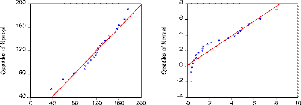
4.2.3Normality Graphs


OP OUEP

Quantiles of OP Quantiles of OUEP
Figure 13: Normality Graphs
The normality of data showed that data is well modelled and is
normally or evenly distributed. The graph 11 shows the distribution of
normality of each of the variables of this study. The red line in each data is
the ideal location of the data points. The blue points show the actual position
of each data point in the study. The graphs in the following section show that
all the data in this study is normally distributed.
4.2.4Regression Analysis
Regression analysis is a statistical analysis which allows the
researchers to examine the relationship that holds between a dependent and the
independent variables that are included in the research i.e. this analysis
equips the researcher to examine the relationship between two or more
variables of interest. In the table 3, given below the horizontally presented
variables are the dependent variables which include GDPG, UNR, AGG, MAG and PCI
while the vertical column shows independent and control variables; OER is
independent and OP and OUEP are control variables of this research. The table
shows that increasing OER by one unit increases GDP by 47.2%, decreases UNR by
1.4%, increases AG by 54.9% and PCI by 58.6%. However, UER does not increases
or decreases AGG significantly since its p-value is above 0.05. As for relation
with OP, it is significant for GDPG, causing increase of 15.5%, for MAG,
increasing it by 13.3% and with PCI by increasing it by 14.7 %. Finally, for
OUEP is significantly related with UNR, causing decrease of 12.4%, MAG causing
increase of 182 and with PCI increasing it by 180. The C value row is the
values taken constants in each relationship.
Table 5: Regression Analysis
|
Independent variables
|
Dependent Variable
|
|
|
|
|
GDPG UNR AGG
|
MAG
|
PCI
|
|
|
Coef. P-value Coef. P-value Coef.
|
P-value Coef.
|
P-value Coef.
|
P-value
|
|
OER
|
0.472 0.019
|
-0.014 0.044
|
0.065
|
0.730
|
0.549
|
0.003
|
0.586
|
0.007
|
|
OP
|
0.155 0.007
|
-0.003 0.849
|
-0.028
|
0.586
|
0.133
|
0.008
|
0.147
|
0.013
|
|
OUEP
|
1.680 0.05
|
-0.124 0.000
|
-0.637
|
0.443
|
1.824
|
0.019
|
1.805
|
0.045
|
|
C
|
-23.754 0.003
|
02.383 0.000
|
6.382
|
0.387
|
-20.83 0.003
|
-29.34 0.001
|
|
R-squared
|
0.610947
|
0.751185
|
0.033768
|
0.687175
|
0.637062
|
|
Adjusted R-squared
|
0.546105
|
0.709716
|
-0.127270
|
0.635038
|
0.576573
|
|
S.E. of regression
|
6.512862
|
0.241497
|
6.600171
|
5.768792
|
6.827395
|
|
Sum squared resid
|
763.5128
|
1.049774
|
784.1206
|
599.0212
|
839.0398
|
|
Log likelihood
|
-70.23241
|
2.250493
|
-70.52537
|
-67.56345
|
-71.27002
|
|
F-statistic
|
9.422064
|
18.11431
|
0.209690
|
13.18006
|
10.53176
|
|
Prob(F-statistic)
|
0.000580
|
0.000011
|
0.888360
|
0.000086
|
0.000316
|
|
Durbin-Watson stat
|
1.90156764
|
1.050904
|
2.887775
|
1.937742
|
1.181318
|
The lower portion of the above table show several
characteristic values calculated for the variables. Statistics shows the
variance values between the mean of sample and the variance in the sample. The
squared and adjusted r-squared values are measure for variation proportion in
data. Sum squared resid value is the sum of estimated error in the values. The
Durbin Watson (DW) statistic is a test which checks the residuals of data for
autocorrelation. The values for this test are to lie between 0 and 4. Values
from 02 indicate a positive autocorrelation in the variables and values from
2-4 show that a negative autocorrelation is present. The table shows values for
all are almost lying around 3, therefore this data is showing positive
correlation.
| 


