Impact of tax revenue on economic growth in Rwanda from 2007-2017

4.8 DIAGNOSTIC TESTS

In econometrics analysis the diagnostic tests are important to check whether the assumptions of tradition regression are confirmed.

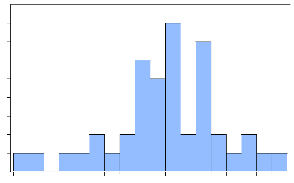
These tests included Normal distribution test, Heteroscedasticity test, Autocorrelation test and Stability test.

4.8.1 NORMALITY TEST

The hypothesis test is as follow

Ho: The residuals are normal distributed

H1 : The residuals are not normal distributed

The null hypothesis is rejected at 10% level of significant

⁴

²

⁹

⁸

⁷

⁶

⁵

³

¹

^{Series: Residuals}

^{Sample 2007Q1 2017Q4}

^{Observations 44}

^Mean ^Median ^Maximum ^Minimum ^Skewness ^Kurtosis ^Jarque-Bera ^Probability

P a g e 40 | 48

Figure 1: Normality test results

Source: Author's computation (2019) by Eviews 8

^{Std. Dev.}

^{2.88e-16 0.003337 0.071187 -0.094099 0.036401 -0.499066 3.414288}

^2.141154

^0.342811

Since the p-value 0.3462811 is greater than 10% level of significance, we fail to reject the null hypothesis that the error term is normally distributed at 95 % confidence interval and conclusion made that the error term is normally distributed.

4.8.2 SERIAL CORRELATION LM TEST

Table 12: Serial correlation LM Test

Breusch-Godfrey Serial Correlation LM Test:

F-statistic 1.188804 Prob. F(1,35) 0.2830

Obs*R-squared 1.379702 Prob. Chi-Square(1) 0.2402

Source: Eviews 7,2019

Table 4.10 reports the results of the first diagnostic test of autocorrelation. The null hypothesis (Ho) claims that there is no autocorrelation while the alternative hypothesis (H1) claims the opposite. The decision rule states that the null hypothesis (H0) should be rejected if the p-value of observed R-squared is less than the 0.05 level of significance. Hence, there is no presence of serial correlation in the estimated model, since the p-value of the observed R-squared is 0.2402 which is greater than the 0.05 level of significance.

4.8.3 HETEROSCEDASTICITY TEST

Table 13: Heteroscedasticity Test result

Heteroscedasticity Test: Breusch-Pagan-Godfrey

F-statistic	0.919697	Prob. F(8,33)	0.5129
Obs*R-squared	7.657008	Prob. Chi-Square(8)	0.4677
Scaled explained SS	19.22575	Prob. Chi-Square(8)	0.0137
Source: Eviews 7,2019

Table 4.13 shows the results of the second diagnostic test of serial correlation. the null hypothesis (Ho) claims that residuals are homoscedasticity and the alternative hypothesis claims that the residuals are heteroscedastic and thus the variance is not constant. The rejection rule states that the null hypothesis should be rejected if the probability value of observation R-squared is less than the 0.05 level of significance. Since the probability of Chi-Square of 0.2402 is greater than 0.05, the test fails to reject the null hypothesis of constancy of variance among the residuals in the model, and thus are deemed to be homoscedastic.

4.8.4 STABILITY OF THE MODEL

^20 ^15 ^10 ^5 ^0 ^-5 ^-10 ^-15 ^-20
	^2009 2010 2011 2012 2013 2014 2015 2016 2017
				^CUSUM 5% Significance

Figure 4. 2 cumulative sum model stability

Source: Author's computation (2019) by Eviews 8

By analyzing the above graph, it was clear that the model is stable because the navigating blue line of graph does not cross the borders (the straight lines represent critical bounds at 5% significance level); this indicates that the GDP of Rwanda have been moving in a stable way from 2007 to 2017

P a g e 41 | 48