Image to image translation with generative adversiale networks (translation of satelite image to Google maps image )

Academic Year 2021/2022

People's Republic of Algeria Ministry of Higher Education and Scientific Research Universite Hassiba Benbouali de Chlef

Faculty: Exact Sciences and Computer Science
Department: Computer Science

THESIS FOR OBTAINING BACHELOR'S DEGREE IN COMPUTER

SCIENCE

presented by :

Chaki Ilyas

Souna Abdelazize

Image to Image Translation with Generative

Adversarial Networks. (Translation of

Satellite Images to Google Maps Images.)

Defended on 12/06/2022 before the jury:

Mr. Ahmed Abbache Supervisor

President Examiner

Contents

introduction 1 Artificial Intelligence 1.1 Machine Learning			vii 1 1
		1.1.1 What is learning	1
		1.1.2 Categories of learning	2
		1.1.3 Limitations	2
		1.1.4 Deep Learning	2
		1.1.4.1 Deep Neural Concepts	4
		1.1.4.2 Deep neural networks	4
		1.1.4.3 Error functions	5
		1.1.4.4 Optimization algorithms:	6
		1.1.4.5 Deep Neural Network Variants	7
	1.2	Natural Language Processing	9
		1.2.1 What is Language?	9
		1.2.2 Why Natural Language Processing?	9
		1.2.2.1 Communication	10
	1.3	Computer Vision	10
		1.3.1 what is computer vision	10
		1.3.2 Convolution neural network(CNN)	10
		1.3.2.1 CNN's concepts .	12
	1.4	Knowledge Representation	12
	1.5	automated reasoning	13
	1.6	robotics	13
		1.6.1 Aspects of robotics .	13
	1.7	Conclusion	13
2	Generative Modeling		14
	2.1	Representation Learning	14
		2.1.0.1 Supervised Representational Learning	14
		2.1.0.2 Unsupervised Representational Learning	15

ii

		CONTENTS
	2.2 2.3	What is generative Modelling 2.2.1 Generative Models 2.2.1.1 AutoEncoders 2.2.1.2 Variational AutoEncoders Generative Adversarial Networks	15 16 16 17 18
		2.3.1 What are Generative Adversarial Networks	18
		2.3.2 Generative Adversarial Network model	18
		2.3.2.1 The Generator Model	19
		2.3.2.2 The Discriminator Model	19
		2.3.3 Generative Adversarial Network Architectures	19
3	The Pix2Pix Model		21
	3.1	Image to Image Translation	21
		3.1.1 Pix2pix model	22
	3.2	The U-net Model	23
		3.2.1 The Unet-Generator Model	23
		3.2.2 The Markovian Discriminator	24
		3.2.3 The Model Loss Function	24
	3.3	Conclusion	25
4	Project Implementation		26
	4.1	Tooling	26
	4.2	Conception	28
	4.3	The Maps Dataset	28
	4.4	Generator Implementation	29
	4.5	Discriminator Implementation	30
	4.6	Pix2Pix Implementation	31
	4.7	Model Training	31
	4.8	Model Evaluation	32
	4.9	Conclusion	32

Listings

4.1	encoder_block	29
4.2	decoder_block	29
4.3	generator	29
4.4	encoder_block	30
4.5	decoder_block	31
4.6	decoder_block	31

List of Figures

1.1 neuron / Source[26] 3

1.2 artificial neuron / Source[18] 3

1.3 artificial neural network / Source[2] 3

1.4 feed forward neural network / Source[14] 7

1.5 radial basis neural network [20] 8

1.6 modular neural network / Source[19] 8

1.7 recurrent neural network / Source [3] 9

1.8 computer vision architecture / Source[7] 10

1.9 convolution operation / Source [15] 11

2.1 generative modeling in the landscape of artificial intelligence / Source[1] 15

2.2 AutoEncoder architecture / Source[21] 16

2.3 variational distribution / Source[22] 17

2.4 fake faces generated using cycle GAN / Source [25] 18

2.5 basic GAN architecture / Source[1] 19

2.6 conditional gan architecture / Source [1] 20

3.1 style transfer / Source [25] 22

3.2 unet / Source[1] 23

3.3 Markovian discriminator / Source [1] 24

4.1 python logo / Source[27] 27

4.2 keras logo / Source[11] 27

4.3 Tensor Flow logo / Source[4] 28

4.4 Tkinter symbol /Source [5] 28

4.5 Examples from the data set 29

List of Tables

1.1	Types of learning	2
1.2	Deep Learning Concepts	4
1.3	Activation Functions	5
1.4	error Functions	6
1.5	optimization algorithms	7
1.6	Deep Learning Concepts	12

acknowledgement

We would love to take this part to show appreciation for everyone who helped directly or indirectly in making this project. First i will start with Vincent Kasozi who first inspired us.

i would love to thank him for being our guide and a good friend

Thanks to Mr.Ahmed Abbache for the opportunity he gave us and for being extremely patient with the process.

Thanks to Souna Abdelazize for accepting the risky offer of taking this project even when we knew so little about the domain. Thanks to the author/creator of every resource that i've used ,the contributions

you'll make is appreciated

I'm trying to make this list as short as possible so i will give a quick acknowledgement to Douba abdrezzak,Otmani Sadiq,Oueldja Mohammed amine for helping with the web part.

introduction

The desire to create is one of the deepest yearnings of the human soul.

Dleter F.Uchtdorf

Mapping technology is one one of the most used technologies in the last couple years ,with the ever growing need for localisation and navigation, there are still weak mapping in certain parts of the world this may require creating efficient maps for various future applications, this will require new efficient and fast way of generating good maps ,the manual process of collecting data and using it for making maps can be costful,Google Maps works with 1,000 third party sources from around the world to collect the data necessary to create accurate maps. in this project we will introduce a solution for automating this process using an advanced deep learning architecture. Artificial intelligence is a

vast field regrouping the humanity quest for replicating and surpassing our intelligence, ever since the first imagination of artificial intelligent entities we came a long way. one of the most impressing qualities of humans is our creativity , this led to a desperate search for a way of creating efficient generative models . In this project we will go through the implementation of a Satellite to map

image translator this style transfer is considered as a generative task ,this will lead to using Generative adversarial networks(GANs), in the first chapter we will introduce the domain of artificial intelligence ,and talk briefly about machine learning and deep learning ,next in the second chapter we will talk about generative modeling as leading to generative adversarial networks and a particular GAN named pix2pix will be used ,in the last chapter we will go through the code implementation.

1

Artificial Intelligence

Introduction

h Machine Learning

h Natural Language Processing h Computer Vision

h Knowledge Representation h Automated Reasoning h Robotics

The Turing test, proposed by Alan Turing (1950), was designed as a thought experiment that would sidestep the philosophical vagueness of the question «Can a machine think?» A computer passes the test if a human interrogator, after posing some written questions, cannot tell whether the written responses come from a person or from a computer.

1.1 Machine Learning

For the last two decades Machine Learning became one of main fields in computer science due to the ever growing computing power ,and the availability of more and more data ,the need to a smart way of data analysis.

Definition 1.1

the development of computer systems able to learn using algorithms and statistical models to analyze and draw inferences in data. [23]

?

1.1.1 What is learning

Learning is the process of gaining knowledge or skill.

2

1.1 Machine Learning

Definition 1.2

?

Learning is the performance's improvement in a particular task with respect to experiance.

1.1.2 Categories of learning

There are three main types of machine learning:

Index Task Explanation

1 Supervised Learning	it consists of an outcome predicted from a given set of independent variables,we us these variables to create a function that best fit the given data ,we keep on modifying the function until it reaches the desired. Hierarchical clustering K-means clustering [10]
2 Unsupervised Learning		in this algorithm there is no outcome ,it is used for clustering data based. Examples for unsupervised learning :apriori algorithm,k-means etc Reinforcement Learning: the machine is trained to make a certain decision by being exposed to the environment and learn from past experiences [10].
3 Reinforcement Learning			In reinforcement learning, an agent interacts with its environment and periodically receives awards that reflect how well it is doing at its task. Reinforcement learning is distinct from "just solving a Markov decision process (MDP)" since the MDP is not presented to the agent as a problem to solve; the agent is in the MDP. It does not know the model of transformation or the reward mechanism, and to learn more [10].

Table 1.1: Types of learning

1.1.3 Limitations

Machine learning is notorious for it'difficult features extraction part, in machine learning that'usually done by the designer ,another limitation would be the inability to create complex patterns for complex data patterns,deep learning solve this two fatal flaws.

1.1.4 Deep Learning

Inspired by how the human brain works, tried to reverse engineer the neurons 1.1 in our central nervous system led to the creation of artificial neuron 1.2 ,stacking this neurons together allows the mapping of more complex data also called Artificial Neural networks (ANN) [8] 1.3.

1.1 Machine Learning

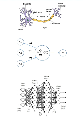
Figure 1.1: neuron / Source[26]

Figure 1.2: artificial neuron / Source[18]

Figure 1.3: artificial neural network / Source[2]

3

4

1.1 Machine Learning

as illustrated in the figure 1.2 there is a main processing part named neuron that takes an input X1,X2,X3...Xn do a processing and fires an output Y ,this is similar to what happens inside our brains. stacking this neurons together forms a network that we can divide into three main parts:

1.1.4.1 Deep Neural Concepts

Index Concept Explanation

1 Activation Function also known as transfer learning,a function that takes the weighted sum

and produced on outcome based on the nature of the function [8]: linear activation function

non linear activation function

2 Error functions a function used for the task of evaluating the network performance ,a

measure of how wrong the network is [8].

3 Optimization in the learning process optimization algorithms are used to minimize

algorithms the error by finding the optimal weights.

4 Batch a way of making networks faster by re-scaling the data ,giving a mean

Normalization of zero and a standard deviation of one [8].

5 Dropout turning off a percentage of the neurons that make up certain layers during

a particular forward or backward pass, it is used to prevent over-fitting [8].

Table 1.2: Deep Learning Concepts

1.1.4.2 Deep neural networks

Deep neural networks or Artificial neural network (ANN) can be divided into three main parts: The input layer:we feed the attribute to the nodes of the first layer.

The hidden layer :each node in the hidden layer takes it's input from the previous layer which is the weighted sum of the outputs of the previous layer given by the expression:

n

_X WiXi (1.1)
i=1

the neuron apply a function of the weighted sum ,this function is called the activation function 1.3:

f(

_Xn i=1

WiXi) (1.2)

The output layer:the nodes of the output layer takes the input from the last hidden layer and apply it's own activation function

Definition 1.3

it is a measure of how accurate the prediction is compared to the correct solution,the lower the error the better the performance. [8]

?

5

		1.1 Machine Learning
Index	Concept	Explanation
1	sigmoid function	1 f(x) =	(1.3)
		1 + e-x
2	ReLU	f(x) = max(0,x)	(1.4)
3	Leaky ReLU	f(x) = max(0.1x, x)	(1.5)
4	Softmax	exp(Zi)	(1.6)
		softmax(Zi) = P j exp(Zj)
5	Hyperbolic Tangent (Tanh)	(e^x- e-x)	(1.7)
		f(x) = (e^x+ e-^x)

Table 1.3: Activation Functions

· Note the process of calculating the output of every layer and passing it to the next layer is called Feed-Forward and it boils down to matrices multiplication.

1.1.4.3 Error functions

Error functions 1.4 is a measure of how far a prediction is from the right answer.

6

		1.1 Machine Learning
				Index
Concept		Explanation		1
Mean error(MSE)	square	it takes the average of the squared sum of all the errors: 1 E(W, b) (ày - = XN yi)^2	(1.8)
Mean error(MSE)	absolute	it takes the average of the absolute valeu of the sum of all the 1 E(W,b) |(ày - = XN	errors: (1.9)
Binary entropy:	cross-	it is mostly used in classification problems: E(W,b) = - Xm yilog(pi) i=1	(1.10)

Table 1.4: error Functions

1.1.4.4 Optimization algorithms:

in order to improve the performance of the network we need to minimize the error and find the optimal weights ,this process of framing a problem and trying to minimize a value is called optimization.

Definition 1.4

optimization algorithms are a group of algorithms that use mathematical tools in order to optimize weights and reach optimal performance in neural networks. [8]

?

these are examples for optimiztion algorithms 1.5

7

1.1 Machine Learning

Index Concept Explanation

1 Batch gradient in this algorithm we use batchs of data to update the weights iteratively

descent(BGD): in order to descent the slope of the curve until we reach the minimal

error.

dE

LWi = -á (1.11)
dWi

Wnext-step = Wcurrent + L (1.12)

2 Stochastic gradient stochastic is just a fancy way to say random, this algorithm uses random

descent SGD): instances of the data instead of the entire batch ,this gives it the advantage
of being faster than BGD,it is vastly used in deep networks.

Table 1.5: optimization algorithms

1.1.4.5 Deep Neural Network Variants

Feed-forward neural networks: it is the most basic form of neural networks where the flow only occurs from the input layer, they only have one layer ,or at most one hidden layer,in this architecture there is no back-propagation technique,they are usually used in face recognition applications1.4

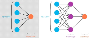
Figure 1.4: feed forward neural network / Source[14]

Radial basis function neural networks: this networks have preferably two layers,the relative

distance from any point to the center is calculated and the same is passed to the next layer 1.5

8

1.1 Machine Learning

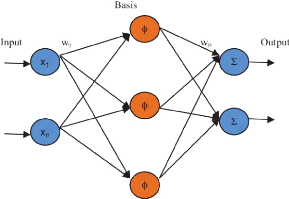
Figure 1.5: radial basis neural network [20]

Multi layer perceptron(MLP): these networks usually have more than three layers with fully connected nodes this architecture is usually used for classifying data and speech recognition and various other applications 1.3

Modular neural networks: this architecture is a combination of smaller networks that serve to achieve a common target ,which is very helpful in breaking a big problem into small pieces 1.6

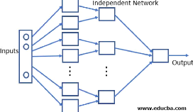
Figure 1.6: modular neural network / Source[19]

Recurrent Neural Network: This architecture is unique for it's use of loops where the output of one neuron is fed back to the same neuron as an input allows the predicting of the output and the creation of small state memory which is useful for video and audio applications 1.7

1.2 Natural Language Processing

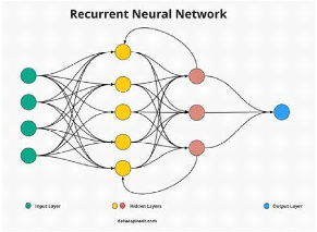
Figure 1.7: recurrent neural network / Source [3]

1.2 Natural Language Processing

Natural language processing (NLP) is a sub-field of linguistics, computer science, and artificial intelligence concerned with the interactions between computers and human language, in particular how to program computers to process and analyze large amounts of natural language data. The goal is a computer capable of "understanding" the contents of documents, including the contextual nuances of the language within them.

Definition 1.5

4

1.2.1 What is Language?

Noam Chomsky gives the following definition to languages: Definition 1.6

language is the inherent capability of native speakers to understand and form grammatical sentences. A language is a set of (finite or infinite) sentences, each finite length constructed out of a limited set of elements. This definition of language considers sentences as the basis of a language. -Noam Chomsky-

4

9

1.2.2 Why Natural Language Processing?

Natural language processing helps computers communicate with humans in their natural language,NLP makes it possible for computers to read text, hear speech and interpret it.

10

1.3 Computer Vision

1.2.2.1 Communication

communication can be defined as the act of interaction between two entities , in the context of Natural Language processing it's the interaction between humans and machines

1.3 Computer Vision

1.3.1 what is computer vision

inspired by the architecture of the vision systems in humans and animals ,we create computer vision by using a sensing device and a interpreting device as illustrated in figure 1.8 in the scope of

Figure 1.8: computer vision architecture / Source[7] this project we will focus on the interpreting part.

· Note traditional Multi layer perceptron network have are fully connected ,means each node is connected to every and each neuron in the next and previous layer with can lead to an explosion in the number of weights when the number offeatures is height ,this will be a problem when we apply it on computer vision. each pixel in an image will be a feature ,in an grey scale 256*256 image will produce 65,536 feature meaning millions of weights ,this will only increase exponentially when we add RGB images with more dimensions,for this exact purpose we use Convolution neural network(CNN).

1.3.2 Convolution neural network(CNN)

in mathematics convolution is the operation of two function to produce a third function, in CONV we multiply each pixel in the image with the corresponding weight in the conv matrix illustrated in figure 1.9 :

weighted - sum = X1W1 + _X2W2 + _X3W3 + ....X_nW_n + b (1.13)

Theorem 1.1

?

Definition 1.7

an architecture in deep learning composed offour parts: Input layer

Convolution layer

1.3 Computer Vision

		Figure 1.9: convolution operation / Source [15]
Fully connected layer Output layer illustrated in figure1.9 [8] 4

Definition 1.8

a Convolution layer(Conv) is a group of matrix that slide over the image to extract features using convolution. [8]

4

11

the task of classification with CNN runs through a pipeline of two main steps:

Feature extraction: it is done by the convolutional layer ,in this phase the network takes all the necessary information out of the image ,and removing the unnecessary complexities. Classification: this phase is usually done by MLP with a sigmoid function at the output layer,it takes the extracted features out of the convolutional layer and output a probability.

· Note CNN architecture is very useful when it comes to conserving the spatial features,also getting rid of the unnecessary informations.

1.4 Knowledge Representation

1.3.2.1 CNN's concepts:

Index Concept Explanation

1 stride Stride is a component of convolutional neural networks, or neural

networks tuned for the compression of images and video data. Stride is a parameter of the neural network's filter that modifies the amount of movement over the image or video. For example, if a neural network's stride is set to 1, the filter will move one pixel, or unit, at a time. The size of the filter affects the encoded output volume, so stride is often set to a whole integer, rather than a fraction or decimal.[13]

2 pooling Pooling layers provide an approach to down sampling feature maps by

summarizing the presence of features in patches of the feature map. Two common pooling methods are average pooling and max pooling that summarize the average presence of a feature and the most activated presence of a feature respectively.[13]

3 kernel as mentioned before ,convolutional operation is done by a group of

matrix ,kernel is just a fancy name for matrix ,the values of the kernel are initialized randomly than we adjust them with back-propagation.[13]

4 Batch Batch normalization is a technique for training very deep neural

Normalization networks that standardizes the inputs to a layer for each mini-
batch. This has the effect of stabilizing the learning process and dramatically reducing the number of training epochs required to train deep networks.[13]

5 Dropout Dropout is a technique that drops neurons from the neural network or

`ignores' them during training, in other words, different neurons are removed from the network on a temporary basis.[13]

Table 1.6: Deep Learning Concepts

1.4 Knowledge Representation

Definition 1.9

Knowledge-representation is afield of artificial intelligence that focuses on designing computer representations that capture information about the world that can be used for solving complex problems

?

12

semantic nets systems architecture

13

1.5 automated reasoning

frames

rules

ontologies

1.5 automated reasoning

·

Definition 1.10

Automated reasoning is the area ofcomputer science that is apply logical reasoning in computing systems. If given a set of assumptions and a goal, an automated reasoning system would be able to make logical inferences towards that goal automatically.

4

Note Automated reasoning is considered to be a sub-field ofartificial intelligence (AI). yet the methods and implementation of both are unique enough. For example, AI typically uses a type logic called modal logic, which uses classical logic while also expressing modality (possibilities or impossibilities). The phrase AI also has connotations denoting a computer which works like a person, which opposes how automated reasoning works.

1.6 robotics

Definition 1.11

Robotics is a branch of AI, composed of Computer Science,Electrical Engineering, and Mechanical Engineering,used for designing,building , and application of intelligent robots [16].

4

1.6.1 Aspects of robotics:

Robots have mechanical construction, form, or shape designed to accomplish the task designed for.

Robots have electrical components which have the role of powering and controlling the machinery. They contain some level of computer program that determines what, when and how a robot does something.

1.7 Conclusion

in this chapter we introduced some of the concepts and tools to use in this project,we will use CNN as a discriminator for the final model,expanding on this ideas was necessary in the process of creating an understanding of why artificial intelligence and why CNN exactly,next we will bring up the Generative adversarial network,and try to give an intuition of how it works.

2

Generative Modeling

Introduction

h Representational Learning

h Generative Models Taxonomy

h Generative Adversarial Networks

h GAN Training

h Applications of GANs h Conclusion

2.1 Representation Learning

In representation learning, data is sent into the machine, and it learns the representation on its own. It is a way of determining a data representation of the features, the distance function, and the similarity function that determines how the predictive model will perform. Representation learning works by reducing high-dimensional data to low-dimensional data, making it easier to discover patterns and anomalies while also providing a better understanding of the data's overall behaviour.

Representation learning is a class of machine learning approaches that allow a system to discover the representations required for feature detection or classification from raw data. The requirement for manual feature engineering is reduced by allowing a machine to learn the features and apply them to a given activity.[1]

Definition 2.1

?

2.1.0.1 Supervised Representational Learning

Supervised Dictionary Learning

2.2 What is generative Modelling

Multi-Layer Perceptron Neural Networks

2.1.0.2 Unsupervised Representational Learning

Learning Representation from unlabeled data is referred to as unsupervised feature learning. Unsupervised Representation learning frequently seeks to uncover low-dimensional features that encapsulate some structure beneath the high-dimensional input data.

2.2 What is generative Modelling

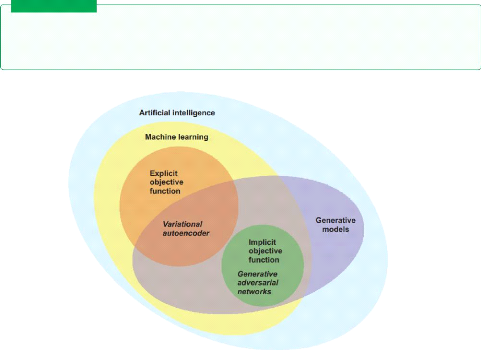
By definition generative modeling is an unsupervised learning task in machine learning that involves automatically discovering and learning the representations or patterns in input data in such a way that the model can be used to generate new examples. [6]

Definition 2.2

?

15

Figure 2.1: generative modeling in the landscape of artificial intelligence / Source[1]

Example 2.1 let's say we want to create realistic looking images of cats, first we will need a dataset containing images of cats ,we call it training data ,we use it to teach our model the rules that govern the appearance of a cat ,the target will be for our model to generate a realistic samples that has never existed before yet still looks real.

· Note The generative model must be probabilistic rather than deterministic ,it can't be simply a fixed calculation like taking the average of all the pixels in the dataset,doing this will produce a deterministic

16

2.2 What is generative Modelling

model which means it's gonna produce the same output every time,the model must have an element of randomness (not generating the same image).

2.2.1 Generative Models

Generative models are deep learning networks with the task of generating data. All these models represent probability distributions over multiple variables in some manner. The distributions that the generative model generates are high-dimensional. For example, in the classical deep learning methodology like classification and regression, we model a one-dimensional output, whereas in generative modelling we model high-dimensional output.

We describe some of the traditional generative networks:

2.2.1.1 AutoEncoders

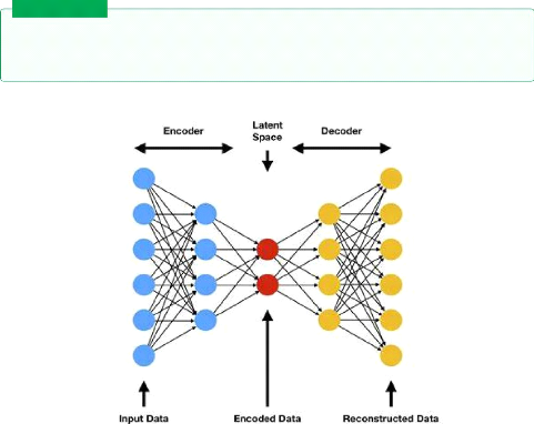
AutoEncoders are a deep learning model usedfor learning a valid representations of unlabeled data ,it is adjusted by trying to regenerate the input data from the encoding [12]. AutoEncoders are composed of two sub models.

Definition 2.3

?

Figure 2.2: AutoEncoder architecture / Source[21]

Encoder takes the data and try to learn a valid simpler representation, in vision tasks it takes an image x fed as a vector of size y and outputs a latent vector with the size z ,from a theory

17

2.3 Generative Adversarial Networks

of information perspective we are trying to find a smaller representation without any loss in the information.

Latent vector(z): it is a smaller representation of the data.

Decoder: takes the latent vector with the size z and output the image x* ,we thrive to make the image x* identical to x.

ïNote The training process ofAutoEncoders is done through one general loss function,in contrast this would no be the case in other architectures we are gonna bring up in the next section.

2.2.1.2 Variational AutoEncoders

The difference between a regular AutoEncoder and a variational AutoEncoder has to do with the latent representation.

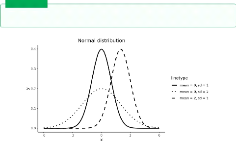
A variational AutoEncoder is a type ofAutoEncoder where the latent vector is represented as a distribution 2.3 with a learned mean and a standard deviation [12]

Definition 2.4

?

Figure 2.3: variational distribution / Source[22]

In the training process of a regular AutoEncoder we learn the values of that vector where as in variational AutoEncoder we need to further learn the parameters of that distribution, this implies that in the decoding process we need to sample from that distribution which means the result will look like the data we fed into the encoder. [12].

· Note The difference for the generating process comesfrom the nature ofthe latent space representation ,in the variational AutoEncoder we get an output that looks something like an example from the dataset,in contrast a regular AutoEncoder the output will be similar to the example we fed.

18

2.3 Generative Adversarial Networks

2.3 Generative Adversarial Networks

Generative adversarial network is a new architecture ,first introduced in 2014 by Ian Goodfellow et al at the International Conference on Neural Information Processing Systems (NIPS 2014). Like any new technology there is no good theories on how to implement the model, yet it achieves remarkable results,in 2019 Nvidia released a realistic fake face images 2.4 ,indistinguishable from real faces using an advanced GAN architecture called Cycle GANs.

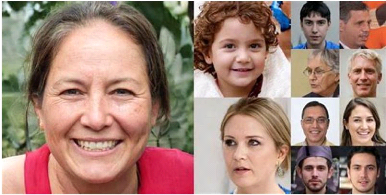
Figure 2.4: fake faces generated using cycle GAN / Source [25]

2.3.1 What are Generative Adversarial Networks

Generative adversarial networks or GANs for short is an approach of generative modeling using deep learning ,it's a way offraming an unsupervised problem of generating data into a supervised problem using two models working together,a generator with the target of generating plausible fake data and the discriminator with the target of classifying fake and real data ,this two sub networks are trained together in an adversarial frame ,in a zero sum game ,where the win of one sub-model is a loss to the other 2.5. [1]

Definition 2.5

?

2.3.2 Generative Adversarial Network model

In a basic GAN architecture the generator takes a random noise vector which is just a vector of random numbers in order to introduce some randomness into the generation process ,the generated is next fed to the discriminator along with a real image from the data set. the training process happens on two cycles ,one for the discriminator and one for the generator

19

2.3 Generative Adversarial Networks

2.3.2.1 The Generator Model

for the generator: in order to train the generator we would need to combine the two models ,the generator generates the image ,the discriminator must classify it as fake ,if so ,it updates the generator

weights in the target of creating fake samples indistinguishable from the samples in the data set.

2.3.2.2 The Discriminator Model

the discriminator takes an image from the data set with label 1 with the target of classifying as real,if the discriminator fails it updates the weights.

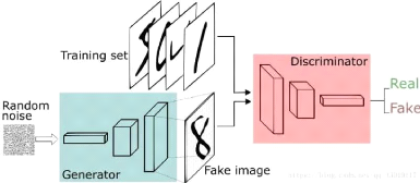
Figure 2.5: basic GAN architecture / Source[1]

· Note GANs differfrom traditional neural networks, in a traditional neural networks there is usually one cost function represented in terms of it's own parameters J(e) ,in contrast in GANs we have two cost functions one for the generator,the otherfor the discriminator ,each of these functions are represented in terms of both the networks's parameters, J^(G)(e^(G), e^(D)) for the generator and J^(D)(e^(G), e^(D)) for the discriminator. the other difference is that traditional neural networks update all the parameters e in the training cycle ,in a GANs there a training cycle for the generator and another for the discriminator in each cycle each network updates only it's weights that means the network updates only a part of what actually makes it's loss.

2.3.3 Generative Adversarial Network Architectures

Even though GAN are a new technology the amount of research that was put into it is huge ,that did lead to the birth of new advanced architecture for various applications,here is a list for some of these applications:

Vanilla GAN :

Deep convolutional GAN : since the Ian Goodfellow paper ,there have been a lot of attempts to fuse CNN as part of the GAN architecture , the reason being CNNs are superior when it comes

20

2.3 Generative Adversarial Networks

to visual tasks , until Radford et al succeded in 2015 in their paper Unsupervised representation learning with deep convolutional generative adversarial networks [17], they used a CNN as both a generator and a discriminator ,here are some guide lines into the implementation of DC-GAN:

strides are preferred over pooling layers in both the generator and the discriminator. Batch normalization should be used in both the generator and the discriminator.

For deep architectures ,fully connected layers should be removed.

For the generator use ReLU activation function expect for the last layer it's preferred to use Tanh rather than sigmoid ,the reason being that images are normalized between (-1, 1) not (0,1).

Conditional GAN: it's a type of GAN introduced by Montreal university student Mehdi Mirza and Flickr Al , where the the generator and the discriminator are conditioned with an information,this information can be a anything, a label,set of tags,a written description etc 2.6 .

Figure 2.6: conditional gan architecture / Source [1]

· Note in the scope of the explanation of the C-GAN,we will consider the auxiliary information to be a label,just for simplicity.

Stack GAN: the translation of a text to a image is a challenging task ,the GAN architecture built for this task is called Stack GAN short for stacked generative adversarial networks ?? introduced is the paper StackGAN:Text to Photo realistic image synthesis with stakced

generative adversarial networks,this network is composed of two GANs stacked on top of each other ,each GAN has a specific role in the creation of the image,the process can be described by the two stages bellow:

Stage 1:turn the text to a primitive sketch of the image

Stage 2: translating the sketch to a full realistic looking image

Super Resolution GAN : the task of augmenting an image into a high resolution image ?? is realized using an architecture called SR-GAN short for super resolution generative adversarial networks ?? introduced in the paper photo-realistic single image super-resolution using generative adversarial networks []

3

The Pix2Pix Model

Introduction

h Image to image Translation h The Unet Model

h The Unet Generator Network

h The Markovian Discriminator h The Model Loss Function h Conclusion

Definition 3.1

image to image translation is the controlled conversion of an input image into a target image,image translation is a challenging task that require a hand crafted lossfunction.[12]

?

3.1 Image to Image Translation

inspired by the language translation ,every scene can have multiple representations such as grey scale,RGB, sketch etc the process of translating an image into another domain is called style transfer 3.1

3.2 The U-net Model

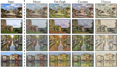
Figure 3.1: style transfer / Source [25]

3.1.1 Pix2pix model

Definition 3.2

Pix2pix is GAN model designed for image to image translation tasks,the architecture was proposed by Philip isola et al in their 2016 paper Image-to-image translation with conditional adversarial networks [9],the pix2pix model is an implementation of the C-GAN where the generation of the image is conditioned on a given image.

?

In the training process of Pix2pix model we give the generator an image to condition the generation process. The output of the generator is next fed to the discriminator along with the original image we fed to the generator, next we provide the discriminator with a pair of real images( original and target image) from the data set. The discriminator is suppose to distinguish real pairs from fake pairs and the generator is suppose to fool the discriminator hence the adversarial nature of the model.

· Note In a Pix2pix model exists two loss functions,the adversarial loss and the L1 loss ,this way we don't only force the generate to produce plausible images for the target domain ,but also to generate images that are plausible as a transformation of the original image.

L1 loss is the mean absolute difference between the generated image and the expected image

Theorem 3.1

_Xi= 1 i=n

|àyi - yi| (3.1)

?

22

23

3.2 The U-net Model

3.2 The U-net Model

First introduced by Philip isola et al in their paper Image-to-image translation with conditional adversarial networks in 2016 [9] ,The U-net ?? is an implementation of the Pix2pix model where the generator in a U-Net model and the discriminator is a Markovian discriminator also known as a patch GAN ,this network proved superior performace on the image to image translation tasks,

3.2.1 The Unet-Generator Model

U-Net is a model 3.2 first build for semantic segmentation. It consists of a contracting path and an expansion path. The contracting path is a typical architecture of a convolutional network. It consists of the repeated application of two 3x3 convolutions, each followed by a ReLU and a 2x2 max pooling operation with stride 2 for downsampling. At each downsampling step we double the number of feature channels. Every step in the expansive path consists of an upsampling of the feature map followed by a 2x2 convolution that halves the number of feature channels, a concatenation with the correspondingly cropped feature map from the contracting path, and two 3x3 convolutions, each followed by a ReLU. At the final layer a 1x1 convolution is used to map each 64-component feature vector to the desired number of classes. In total the network has 23 convolutional layers. [1]

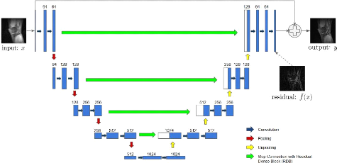
Figure 3.2: unet / Source[1]

· Note You can notice a similarity between the U-net generator and a Encoder network ,the difference is the skip connection between the down-sampling and the up-sampling layers. To gain further intuition on why using a U-Net as a generator for an image to image translation

24

3.2 The U-net Model

task ,we should look at the depth of we are trying to do ;for image to image translation we need to conserve the important feature of the image and use them to create a representation of that image in the target domain, the bottle- neck of the U-Net can be seen as a simple representation of all the image features we extracted using the down-sampling layers, we use those exact features to build our target image through the up-sampling layers.

3.2.2 The Markovian Discriminator

The Markovian discriminator 3.3 also known as a Patch discriminator, a discriminator in a U-Net model takes an the generator paired with the expected image,but different from a regular discriminator classifies patches of the image instead of the entire image.

... We design a discriminator architecture -wich we term a Patch GAN - that only penalizes structure at the scale of patches.This discriminator tries to classify if each N * N patch in a image is real or fake.We run this discriminator convolutionally across the image ,averaging all responses to provide the ultimate output of D

-Image-to-image translation with conditional adversarial networks- [9]

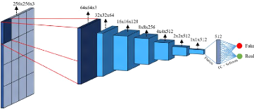
Figure 3.3: Markovian discriminator / Source [1]

ï Note In the original paper [9] ,Philip Isola et al used a patch of 70 * 70,after proving superior performance.

3.2.3 The Model Loss Function

the U-Net uses a combination of the regular adversarial loss and a L1 loss that describe the difference between the generated and the expected image using the absolute mean euror ,in the original paper [9] they used a À = 100 :

loss = adversarialloss + À * L1 (3.2)

25

3.3 Conclusion

· Note The choice of ë = 100 can be seen as a representation of how likely it is to generate any image in the target image compared to generating the exact image we want.

3.3 Conclusion

This chapter was an explanation of the architecture we are gonna use in this project ,U-Net is a complex architecture that uses the concepts we explained in the previous chapters, gaining an understanding about those will help to further understand the code ;next chapter will be a documentation of the project implementation

4

Project Implementation

h Tooling

h UML conception

h The Maps Dataset

h Generator Implementation

h Discriminator Implementation

Introduction

h Pix2Pix Implementation h Model Training h Model Evaluation h Conclusion

4.1 Tooling

In the scope of this project we used a couple tools in both the conception and the implementation ,next we will go into a brief explanation of each tool and what we used it for:

Python: Python is a high-level, interpreted, general-purpose programming language. the design philosophy of python emphasizes code readability with the use of significant indentation.python supports multiple programming paradigms, including structured (particularly procedural), object-oriented and functional programming.

4.2 Conception

Figure 4.1: python logo / Source[27]

Keras:Keras 4.2 is an open source library that gives a Python's interface of Artificial Neural Networks ,Keras can be seen as an interface for TensorFlow library.

27

Figure 4.2: keras logo / Source[11]

Tensorfiow: TensorFlow 4.3 is an open-source software library for machine learning and artificial intelligence. It can be used across a range of tasks but it particularly focus on training deep neural networks.

Tkinter 4.4 :tkinter is a way in Python to create Graphical User interfaces (GUIs),tkinter is included in all standard Python Distributions. This Python framework provides an interface to the Tk toolkit and works as a thin object-oriented layer on top of Tk. The Tk toolkit is a cross-platform collection of `graphical control elements' for building application interfaces.7

28

4.2 Conception

Figure 4.3: Tensor Flow logo / Source[4]

Figure 4.4: Tkinter symbol /Source [5]

4.2 Conception

To further give a intuitive on the code implementation we will use the UML and particularly the class diagram to describe the structure of the model and the inner interaction between the sub-models.

4.3 The Maps Dataset

the maps data set contain two folders for the training and valuation data, the dataset for the pix2pix model is a couple of the source image(satellite image) and the target image(map image) 4.5 , in the implementation of the code we first unpack the data set then load it ,we feed the satellite image to the generator to transfer it to a map image,then we feed the generated image along with the original sattelite image to the discriminator ,then we feed a real data couple to train the discriminator ,for further explanation look at the previous chapter. here are some example of the used samples 4.5

29

4.4 Generator Implementation

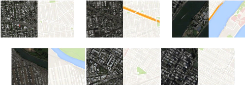
(a) example 1 (b) example 2 (c) example 3

(d) example 4 (e) example 5 (f) example 6
Figure 4.5: Examples from the data set

4.4 Generator Implementation

Listing 4.1: encoder_block

1 def define_encoder_block(layer_in, n_filters, batchnorm=True):

2 init = RandomNormal(stddev=0.02)

3 g = Conv2D(n_filters, (4,4), strides=(2,2), padding='same',kernel_initializer=init

)(layer_in)

4 if batchnorm:

5 g = BatchNormalization()(g, training=True)

6 g = LeakyReLU(alpha=0.2)(g)

7 return g

Listing 4.2: decoder_block

1 def decoder_block(layer_in, skip_in, n_filters, dropout=True):

2 init = RandomNormal(stddev=0.02)

3 g = Conv2DTranspose(n_filters, (4,4), strides=(2,2), padding='same',

kernel_initializer=init)(layer_in)

4 g = BatchNormalization()(g, training=True)

5 if dropout:

6 g = Dropout(0.5)(g, training=True)

7 g = Concatenate()([g, skip_in])

8 g = Activation('relu')(g)

9 return g

Listing 4.3: generator

1 def define_generator(image_shape=(256,256,3)):

2 init = RandomNormal(stddev=0.02)

3 # image input

4 in_image = Input(shape=image_shape)

30

4.5 Discriminator Implementation

5 # encoder model: C64-C128-56-C512-C512-C512-C512-C512

6 e1 = define_encoder_block(in_image, 64, batchnorm=False)

7 e2 = define_encoder_block(e1, 128)

8 e3 = define_encoder_block(e2, 256)

9 e4 = define_encoder_block(e3, 512)

10 e5 = define_encoder_block(e4, 512)

11 e6 = define_encoder_block(e5, 512)

12 e7 = define_encoder_block(e6, 512)

13 # bottleneck, no batch norm and relu

14 b = Conv2D(512, (4,4), strides=(2,2), padding='same', kernel_initializer=init)(e7)

15 b = Activation('relu')(b)

16 # decoder model: CD512-CD1024-CD1024-C1024-C1024-C512-56-C128

17 d1 = decoder_block(b, e7, 512)

18 d2 = decoder_block(d1, e6, 512)

19 d3 = decoder_block(d2, e5, 512)

20 d4 = decoder_block(d3, e4, 512, dropout=False)

21 d5 = decoder_block(d4, e3, 256, dropout=False)

22 d6 = decoder_block(d5, e2, 128, dropout=False)

23 d7 = decoder_block(d6, e1, 64, dropout=False)

24 # output

25 g = Conv2DTranspose(3, (4,4), strides=(2,2), padding='same', kernel_initializer=

init)(d7)

26 out_image = Activation('tanh')(g)

27 # define model

28 model = Model(in_image, out_image)

29 return model

4.5 Discriminator Implementation

Listing 4.4: encoder_block

1 def define_discriminator(image_shape):

2 init = RandomNormal(stddev=0.02)

3 in_src_image = Input(shape=image_shape)

4 in_target_image = Input(shape=image_shape)

5 merged = Concatenate()([in_src_image, in_target_image])

6 d = Conv2D(64, (4,4), strides=(2,2), padding='same', kernel_initializer=init)(

merged)

7 d = LeakyReLU(alpha=0.2)(d)

8 d = Conv2D(128, (4,4), strides=(2,2), padding='same', kernel_initializer=init)(d)

9 d = BatchNormalization()(d)

10 d = LeakyReLU(alpha=0.2)(d)

11 d = Conv2D(256, (4,4), strides=(2,2), padding='same', kernel_initializer=init)(d)

12 d = BatchNormalization()(d)

13 d = LeakyReLU(alpha=0.2)(d)

14 d = Conv2D(512, (4,4), strides=(2,2), padding='same', kernel_initializer=init)(d)

31

4.6 Pix2Pix Implementation

15 d = BatchNormalization()(d)

16 d = LeakyReLU(alpha=0.2)(d)

17 d = Conv2D(512, (4,4), padding='same', kernel_initializer=init)(d)

18 d = BatchNormalization()(d)

19 d = LeakyReLU(alpha=0.2)(d)

20 d = Conv2D(1, (4,4), padding='same', kernel_initializer=init)(d)

21 patch_out = Activation('sigmoid')(d)

22 model = Model([in_src_image, in_target_image], patch_out)

23 opt = Adam(lr=0.0002, beta_1=0.5)

24 model.compile(loss='binary_crossentropy', optimizer=opt, loss_weights=[0.5])

25 return model

4.6 Pix2Pix Implementation

Listing 4.5: decoder_block

1 def define_gan(g_model, d_model, image_shape):

2 d_model.trainable = False

3 in_src = Input(shape=image_shape)

4 gen_out = g_model(in_src)

5 dis_out = d_model([in_src, gen_out])

6 model = Model(in_src, [dis_out, gen_out])

7 opt = Adam(lr=0.0002, beta_1=0.5)

8 model.compile(loss=['binary_crossentropy', 'mae'], optimizer=opt, loss_weights

=[1,100])

9 return model

4.7 Model Training

Listing 4.6: decoder_block

1 def train(d_model, g_model, gan_model, dataset, n_epochs=10000, n_batch=1):

2 n_patch = d_model.output_shape[1]

3 trainA, trainB = dataset

4 for i in range(n_epochs):

5 [X_realA, X_realB], y_real = generate_real_samples(dataset, n_batch, n_patch)

6 X_fakeB, y_fake = generate_fake_samples(g_model, X_realA, n_patch)

7 d_loss1 = d_model.train_on_batch([X_realA, X_realB], y_real)

8 d_loss2 = d_model.train_on_batch([X_realA, X_fakeB], y_fake)

9 g_loss, _, _ = gan_model.train_on_batch(X_realA, [y_real, X_realB])

10

11 # summarize model performance

12 if (i+1) 'f, 1000 == 0:

13 print('>'f,d, d1['f,.3f] d2['f,.3f] g['f,.3f]' 'f, (i+1, d_loss1, d_loss2, g_loss))

32

4.8 Model Evaluation

14 summarize_performance(i, g_model, dataset)

4.8 Model Evaluation

for the evaluation we used the human perspective for it's both efficient and easy ,this method was proposed and used by Ian Goodfellow et al in the original paper Improved techniques for training gans [24] , there are other methods for the evaluation of the network performance ,one being the inception score that uses the inception network to classify the generated images.

4.9 Conclusion

Throughout this project we used the Pix2pix network to implement a translation from satellite images to map images , the first chapter was a introduction to artificial intelligence and machine learning then about deep learning ,then in the second chapter we advanced towards generative modeling and we talked about why it is such a useful architecture, in the same chapter we talked about GAN's and their superior performance in generative modeling ,in the third chapter we spoke on the pix2pix architecture in particular since it`'s the used architecture, in the last chapter we went through the implementation of the code. Since it's introduction by Ian Goodfellow ,generative adversarial networks held great promises ,this is totally understandable for the reason that it represent the creativity form of intelligence and a milestone in the quest of creating general intelligence. The model would generate better results given more training time and data ,so this project can be seen as a prototype and there is a room for improvement. The pix2pix model is also hard to implement cause of it's dataset obligations,the need for a couple of images from the original and the target domain can be realised to a certain degree in the satellite/ map application but is extremely hard for other style transfers,this can be improved using Cycle GAN . I would like this project to be viewed as an example of what GAN's can do ,and for it to serve as an inspiration for people wanting to take on this domain.

Bibliography

[1] Jason Brownlee. Generative adversarial networks with python: deep learning generative models for image synthesis and image translation. Machine Learning Mastery, 2019.

[2] data science central. artificial neural network. [Online; accessed January 9,2022 ]. 2019. uRL: https://www.datasciencecentral.com/the-artificial-neural-networks-handbook-part-1/.

[3] dataaspirant.com. reccurant neural network. [Online; accessed January 12,2022 ]. 2021. uRL: https : / / dataaspirant . com / how - recurrent - neural - network - rnn - works/.

[4] datascientest.com. tensorfiow. [Online; accessed march 14,2022 ]. 2020. uRL: https: // datascientest.com/tensorflow.

[5] e-techno-tutos.com. tkinter. [Online; accessed march 7,2022 ]. 2021. uRL: https:// www.e-techno-tutos.com/2020/12/28/raspberry-tkinter-pour-python/.

[6] David Foster. Generative deep learning: teaching machines to paint, write, compose, and play. O'Reilly Media, 2019.

[7] freecontent.manning.com. computer vison pipeline. [Online; accessed January 12,2022 ]. 2021. uRL: https://freecontent.manning.com/computer-vision-pipeline-part-1-the-big-picture/.

[8] Sunila Gollapudi. ?Deep Learning for Computer Vision? inapril 2019: pages 51-69. iSBN: 978-1-4842-4260-5. Doi: 10.1007/978-1-4842-4261-2_3.

[9] Phillip Isola andothers. ?Image-to-image translation with conditional adversarial networks? inProceedings of the IEEE conference on computer vision and pattern recognition: 2017, pages 1125-1134.

[10] JavaTpoint. What Is Machine Learning: Definition, Types, Applications And Examples. https : / / www . potentiaco . com/ what - is - machine - learning - definition - types-applications-and-examples/. 2021 (accessed march, 8, 2022).

[11] keras.io. keras. [Online; accessed march 14,2022 ]. 2019. uRL: https://keras.io/.

[12] Jakub Langr and Vladimir Bok. GANs in Action (Audiobook). Manning Publications, 2019.

34

BIBLIOGRAPHY

[13] machine learning mastery. A Gentle Introduction to Batch Normalization for Deep Neural Networks. https://machinelearningmastery.com/batch-normalization-for-training-of-deep-neural-networks/. 2019 (accessed January 16, 2022).

[14] medium.com. feed forward neural network. [Online; accessed January 10,2022 ]. 2021. URL: https://medium.com/mlearning-ai/training-feed-forward-neural-network-ffnn-on-gpu-beginners-guide-2d04254deca9.

[15] perso.esiee.fr. convolution. [Online; accessed January 12,2022 ]. 2021. URL: https: // perso.esiee.fr/~perretb/I5FM/TAI/convolution/index.html.

[16] Tutorials point. Artificial Intelligence - Robotics. https://www.tutorialspoint. com/artificial_intelligence/artificial_intelligence_robotics.htm#. 2022 (accessed June, 1, 2022).

[17] Alec Radford, Luke Metz and Soumith Chintala. ?Unsupervised representation learning with deep convolutional generative adversarial networks? inarXiv preprint arXiv:1511.06434: (2015).

[18] researchgate.net. artificial neuron. [Online; accessed January 8,2022 ]. 2019. URL: https: / / www . researchgate . net / figure / The - structure - of - the - artificial - neuron_fig2_328733599.

[19] researchgate.net. modular neural network. [Online; accessed January 11,2022 ]. 2021. URL: https : / / www . researchgate . net / figure / Modular - neural - network - structure_fig4_341628332.

[20] researchgate.net. radial basis neural network. [Online; accessed January 10,2022 ]. 2021. URL: https://www.researchgate.net/figure/Architecture- of- the- RBF-neural-network-RBF-radial-basis-function_fig2_333469185.

[21] researchgate.net. The general autoencoder architecture. [Online; accessed January 14,2022 ].2021.URL: https://www.researchgate.net/figure/The-general-autoencoder-architecture_fig2_328760180.

[22] researchgate.net. variational distribution. [Online; accessed January 14,2022 ]. 2020. URL: https://www.researchgate.net/figure/Variational-Bayes-approximate-posteriors - for - the - regression - model - parameters - and - four _ fig2 _ 227369415.

[23] Stuart J Russell. Artificial intelligence a modern approach. Pearson Education, Inc., 2010.

[24] Tim Salimans andothers. ?Improved techniques for training gans? inAdvances in neural information processing systems: 29 (2016).

[25] whichfaceisreal.com. fake faces using style gan. [Online; accessed february 14,2022 ]. 2019. URL: https://www.whichfaceisreal.com/methods.html.

[26] Wikipedia, the free encyclopedia. neuron. [Online; accessed January 7,2022 ]. 2021. URL: https://ar.wikipedia.org/wiki/%D9%85%D9%84%D9%81:Neuron.svg.

35

BIBLIOGRAPHY

[27] Wikipedia, the free encyclopedia. python. [Online; accessed march 14,2022 ]. 2019. URL: https://fr.m.wikipedia.org/wiki/Fichier:Python.svg.