Hydrological modeling of the Congo River basin: Asoil-water balance approach

UNIVERSITY OF BOTSWANA

Faculty of Sciences
Geology Department
MASTERS PROGRAMME OF HYDROGEOLOGY

HYDROLOGICAL MODELLING OF THE CONGO RIVER BASIN: A SOIL-WATER BALANCE APPROACH

Josué BAHATI CHISHUGI

A Dissertation submitted to the School of Graduate Studies in partial fulfilment of the requirements for the degree of Master of Science (MSc) in Hydrogeology

SUPERVISOR: Dr B.F. Alemaw
2008

DECLARATIONS

I solemnly declare that this work is the result of my own toiling and has never been submitted anywhere for any award.

Signature of Author

Date

Josue BAHATI CHISHUGI

This dissertation has been submitted for examination with my authority as a University supervisor.

Signature of the Supervisor

Date

Dr B.F. ALEMAW

STATEMENT OF COPYRIGHT

No part of this dissertation may be reproduced, stored in any retrieval system, or transmitted in any form or by any means: electronic, mechanical, photocopying, recording, or otherwise, without prior written permission of the Author or the University of Botswana.

ACKNOWLEDGEMENT

To my Parents, brothers and sisters in D.R.Congo for their unlimited love and support through the many years of school;

To my fiancée, Rachel Moiza Maline, for her Love and endurance,

To the German Academic Exchange (DAAD) for the fellowship which enabled us to complete this M.Sc. degree in Hydrogeology;

To my supervisor Dr B.F. Alemaw, for his invaluable help and encouragement, fruitful advice and patience during my introduction to Water Balance Modelling;

To Dr. T.R. Chaoka, the Head of Geology Department, University of Botswana, for his advices and financial support that regenerated my efforts;

To all the Staff member of Geology Department for their advises and supports;

To my Congolese family in Botswana, in particular Madam P. Kampunzu, Dr. Lukusa and His wife, Papa and Maman Mihigo, Prof. Kitenge's family, V. L. Basira, A. Ibrahim, S. Loly, S.M. Oscar, L. Wani, Dr Chantal and Asina;

To Neovitus Shayio, K. Justin and Kaniki, Tina, Adjoa, and many good people I met in Botswana, Geramny and Malawi;

To my graduate colleagues in Batswana, Z. Chiyapo, M. Brighton «The useless Boy», Oteng, Obone, Pricila, Lynette, Haward, Defaru, Lintwe;

I am truthfully grateful and express my thanks.

EPIGRAPHS

Oh God!
Make me strong to overcome my weaknesses, and
Blessed be Your Name forever and ever.
Amen

Dear Parents, My gods!
Despite your insufficiencies,
You showed me the way to School.
I have understood your divinity!
Thanks for your Love and Sacrifices.

Josué B. Chishugi

ABSTRACT

During the last decade African continent has been characterised by a shortage of water, electricity and food due probably to climatic change and mismanagement of the natural resources. The political stability in Central Africa region, the progress in industrial development in southern and the northern Africa gradually increase the need in water for domestic, agricultural, industrial and environmental uses. The second longest river in Africa, contributing with 30% to the African discharge to the Atlantic Ocean, the Congo contains the second largest forest in the world, after the Amazon, sustains the global climate change regulation and ecosystem stability; therefore, the understanding of its hydrology is of grand importance.

In order to understand and evaluate the spatial and temporal distribution of the Congo River Basin (CRB) water balance, a distributed GIS-based hydrological model, namely Hybrid Atmospheric and Terrestrial Water Balance (HATWAB) initially developed by Alemaw (2006) was parameterised and applied to the Congo basin using Rainfall, Potential Evapotranspiration, soils and vegetation information. The model simulates the Soil-water balance model component, namely the Integrated Vertical Moisture Convergence (C), soil moisture (SM), Actual Evapotranspiration (AET) and Runoff (ROF). The spatial distribution of the simulated components correlate strongly with Rainfall patterns, especially in the high rain fed region (Effective Rainfall >1100 mm/year), corresponding to the central part of the equatorial forest, and extending between 5 and -5 degrees of latitude; whereas some disturbances are observed in the lowest rain fed (Effective Rainfall <1000 mm/year) regions of the basin located the south-eastern and the up-north part of the CRB. The Evapotranspiration Ratio (ETR) shows two main climatic regions, ETR close to 1 for region 1 and ETR<7 for region 2, with an intermediate zone between (07<ETR<0.8). The Annual average SM varies between 0 and 400 mm while the actual Evapotranspiration (AET) varies between 400 and 1700 mm/year with highest values on the water bodies. The based-wide gridded runoff (ROF) varies between 0 and 1400 mm/annum with a annual average of 324 mm/a. Flooded wetland areas and swamps are characterised by 0 to 40 mm/a values while highest runoff (> 900mm/a) are computed on the rivers and lakes. The inland grid ROF varies between 50 and 900 mm per year with an average of 324 mm/year. The accumulated ROF computed at the CRB outlet reaches 44700m3/sec, which is within 5% of marginal error compared to the observed discharge of the Congo River.

A supporting script tool (DEMHydro) was developed to extracts the topographic, topologic and hydrologic characteristics of the basin, using Digital Elevation Model (DEM) information.

TABLE OF CONTENTS

DECLARATIONS II

STATEMENT OF COPYRIGHT III

ACKNOWLEDGEMENT IV

EPIGRAPHS V

ABSTRACT VI

TABLE OF CONTENTS VII

LIST OF FIGURES XI

LIST OF TABLES XIII

LIST OF TABLES XIII

LIST OF ABBREVIATIONS, ACRONYMS AND SYMBOLS XIV

LIST OF ABBREVIATIONS, ACRONYMS AND SYMBOLS XIV

CHAPTER ONE 1

1.0	INTRODUCTION OF THE STUDY	1
1.1	Introduction	1
1.2	Statement of problem	1
1.3	Research objectives	2
1.4	Importance of study	2
1.5	Organisation of the thesis	3

CHAPTER TWO 4

2.0 OVERVIEW OF THE STUDY AREA 4

2.1 The Study Area 4

2.2 Physiography 5

2.3 Hydrology 6

2.4 Climate 8

2.5 Soils 10

2.6 Land cover/use and Population density 11

2.7 Geology 13

2.7.1 Basement formation 13

2.7.2 Surface formations 13

CHAPTER THREE 14

3.0 LITERATURE REVIEW 14

3.1 Hydrological models 14

3.2 Water Balance Model approaches 15

3.2.1 Atmospheric Water Balance Studies 16

3.2.2 Soil Water Balance Studies 16

3.2.3 Surface Water Balance Studies 17

3.2.3.1 Water Balances 17

3.2.3.2 Runoff Mapping 18

3.3 Potential evapotranspiration (ETp) and Effective rainfall determination 18

3.3.1 Estimation of Potential Evapotranspiration 18

3.3.1.1 Net radiation 19

3.3.1.2 Mean Relative Humidity 20

3.3.1.3 Wind speed 20

3.3.1.4 Solar radiation 20

3.3.2 Estimation of Effective Rainfall 21

CHAPTER FOUR 23

4.0 METHODOLOGY 23

4.1 Watershed and streams characteristics 23

4.2 Watershed and drainage network Processing Method 23

4.3 DEM-Hydro processing output maps 25

4.3.1 DEM Visualization and areal distribution over elevation 25

4.3.2 Flow direction map 27

4.3.3 Flow accumulation 28

4.3.4 Drainage network extraction and ordering 29

4.3.5 Catchment and Sub-Catchments extraction 30

4.3.6 Overland Flow map 32

4.4 Watershed characteristics 33

4.4.1 Watershed Geomorphology 33

4.4.1.1 Area and length 33

4.4.1.2 Watershed Shape 35

4.4.2 Morphometric Analysis 35

4.4.2.1 Morphometric network topology 35

4.4.2.2 Horton morphometric parameters 36

4.5 GIS-Based Hydrological Model Development 41

4.5.1 Introduction 41

4.5.2 Water Balance Model development procedure 43

4.5.3 Water Balance Model Development 43

4.5.3.1 Atmospheric water balance 43

4.5.3.2 Terrestrial water balance 44

4.5.3.3 Imbalance estimation 45

4.5.3.4 Rainfall-Actual Evapotranspiration-Soil moisture-Runoff modelling 45

4.5.4 Data sets and software 48

4.5.4.1 GIS and geo-referencing procedure 48

4.5.4.2 Meteorological data sets 48

4.5.4.3 Discharge data 50

4.5.4.4 Digital Elevation Model (DEM) and Mask files 50

4.5.4.5 NDVI and vegetation database 51

4.5.4.6 Soil properties 51

4.5.4.7 Software resources 55

CHAPTER FIVE 56

5.0 MODEL APPLICATION, DATA PRESENATTION AND INTERPRE-TATION RESULTS 56

5.1 Generalities on the Model application 56

5.2 Initial soil moisture 56

5.3 Data presentation and Interpretation results 57

5.3.1 Soil moisture (SM) 57

5.3.2 Actual Evapotranspiration (AET) 59

5.3.3 Runoff 60

5.3.4 Simulated sub-watershed and basin-wide runoff 62

5.3.5 Vertical Integrated Moisture Convergence 65

CHAPTER SIX 67

6.0 CONCLUSIONS AND RECOMMENDATIONS 67

6.1 Conclusions 67

6.2 Recommendations 68

REFERENCES 69

APPENDICES 74

APPENDIX 1: METEOROLOGICAL STATIONS COVERING THE STUDY AREA (FROM FAO/UNESCO CLIMWAT DATBASE) 75

APPENDIX 2: SPREADSHEET MODEL FOR THE PENMAN-MONTEITH CALCULATION METHOD OF ETO (AFTER ALLEN ET AL, 1998) 79

APPENDIX 3: CONGO RIVER DISCHARGE DATA AT KINSHASA 82

APPENDIX 4: ATTRIBUTE TABLE FOR DRAINAGE NETWORK ORDERING 84

APPENDIX 5: HORTON STATISTICS FUNCTIONALITY: DEFINITION OF PARAMETERS 85

APPENDIX 6: HORTON MORPHOLOGICAL PARAMETERS AND STATISTICS FOR SUBSEQUENT STRAHLER ORDER 86

APPENDIX 7 PEARSON PRODUCT MOMENT CORRELATION BETWEEN HORTON AND GIUH 87

APPENDIX 8.A. LOCAL WATER BALANCE FOR SELECTED GRID CELLS IN THE
CONGO RIVER BASIN (TABLE) 88

APPENDIX 8.B. LOCAL WATER BALANCE FOR SELECTED GRID CELLS IN THE
CONGO RIVER BASIN (GRAPHS) 90

APPENDIX 9: SEASONAL DISTRIBUTION OF THE CONVERGENCE MOISTURE SAMPLES FOR SELECTED GRID CELLES OVER THE CONGO BASIN (C) 91

LIST OF FIGURES

Figure 1 General Location Map: Position of the study area in Africa 4

Figure 2 The Congo River Basin Elevation System. The high est station elevation is located in the Tanzanian region while the lowest, at the Atlantic Ocean (Note: this elevation grid is derived

from the elevation of the selected 145 meteorological stations falling inside the study area) 6

Figure 3 Mean Discharge Regime of the Congo River Basin at the Kinshasa gauge 7

Figure 4 Monthly discharge of the Congo River (Kinshasa gauge). Mean 1960-1990 7

Figure 5 Meteorological profile of D.R.Congo 9

Figure 6 Long-term mon thly average of Effective Rainfall (1961-1990) at grid cell. 9

Figure 7 Effective rainfall distribution for three selected grids in the Area 10

Figure 8 Congo Basin Agronomic Soils Map. The polygon limit the Congo watershed 11

Figure 9 Vegetation and Land cover and uses over the Congo River Watershed (after World river resources, 2003) 12
Figure 10 Population density distribution over the Congo River Watershed: Basin area 3,730,881 sq.Km, Average Population Density (people per sq.km): 15, Number of large cities (100,000

people). 12

Figure 11 Hydrological Model Classification 14

Figure 12 DEM Processing flow chart: Extraction of Drainage network, Catchment and Horton

Parameters. 24

Figure 13 Areal distribution at different altitude (The area in a logarithmic scale) 25

Figure 14 DEM visualization map for Cental Africa. The defined colored polygone delineated the Congo River basin. 26
Figure 15 D-8 algorithm: Based on the output Flow direction map, the Flow accumulation operation counts the total number of pixels that will drain into outlets (after ILWIS 3.4 Manual)

27

Figure 16 Flow direction map 27

Figure 17 Histogram of Flow Direction for Central Africa 28

Figure 18 Flow Accumulation map; on top: Entire basin, on bottom: A selected area 29

Figure 19 Stream network map masked by the boundary of the Congo River Basin 30

Figure 20 Extracted sub-catchment map in the Congo Basin 31

Figure 21 Merged sub-watershed with stream network and majors outlet of the CRB 31

Figure 22 Longest flow path map overlayed on the sub-watersheds of the CRB 32

Figure 23 Overland flow distribution in the study area 32

Figure 24 Overland flow distribution in the Ouesso sub-watershed 33

Figure 25 Horton morphometric parameters for 4 selected sub-watersheds in the Congo River

37

Figure 26 Strahler order vs. Stream length map 39

Figure 27 General terrestrial Water Balance model structure 42

Figure 28 Rainfall-Runoff simulation model for a single grid cell 42

Figure 29 Functional relationship between soil moisture and Evapotranspiration (ETa is the actual Evapotranspiration, ETp is the potential Evapotranspiration, SM is the soil moisture, FC is the field capacity and WP, the Wilting point 47
Figure 30: Distribution of Clima tic stations in the study area. The study area covers more than

145 stations 49
Figure 31 Rainfall averaged (1961-190) data from 145 stations. 1. Rainfall, 2. Effective Rainfall 49

Figure 32 Mean Annual Potential Evapotranspiration (1961-1990) map 50
Figure 33 Available soil water vs. soil texture showing estimates of field capacity, permanent wilting point and Available water content. S-Sand, SI-Silt, CL-Clay, F-Fine, VF-Very Fine, L-

Loamy (after Levy et al, online) 53

Figure 34 Hydrological Soil types over the basin 54

Figure 35 Soil Field Capacity in the root zone. 54

Figure 36 Hydrological Soil types over the basin 55

Figure 37 Soil moisture correlation with the latitude 57

Figure 38 Mean annual moisture (in mm) over the Congo basin. 58

Figure 39 Season Soil moisture (in mm per season) over the basin. 58

Figure 40 Mean Annual Actual Evapotranspiration over the Congo River basin 59

Figure 41 Season Actual Evapotranspiration over the Congo basin 60

Figure 42 Mean annual runoff over Congo basin (mm/year) 61

Figure 43 The relationship between precipitation and drigged simulated runoff in the CRB 61

Figure 44 Seasonal Runoff grid runoff maps. Top left: December-February, Top right: MarchMay, Bottom Left: June-August, Bottom right: September-November 62
Figure 46 Seasonal and Spatial distribution maps for Vertical Integrated Moisture Convergence (in mm/month) over the Congo River basin. A: December-February, B: March-May, C: JuneAugust, D: Septembre-November (Negative values correspond to the moisture convergence,

positive values correspond to the moisture divergence). 65

LIST OF TABLES

Table 1 River discharge at KINSHASA gauge (after Vorosmarty et al, 1998) 7

Table 2 Effective Rainfall distribution in the Congo Basin 9
Table 3 Land cover distribution in the Congo River basin (after World river resources, 2003).... 11

Table 4 Summarised Statistics for the DEM 26

Table 5 Summarised statistics for the Flow direction grid map in the area of study. 28

Table 6 Sub-wateshed characteristics of the CRB 34

Table 7 Extra cted sub-watersheds areas of the CRB 34

Table 8 Stream numbers and Bifurcation Ratio for sub-watersheds of the Congo River 36

Table 9 Horton Morphometric Parameters for the sub-catchments in the Congo River 38

Table 10 Stream Length Ration for the different sub-catchments in the Congo River 38

Table 11 Stream Ration for the selected subwatershed 39

Table 12 Drainage density for watersheds of the Congo River 40

Table 13 Rooting depth assigned for various soil textures and SCS soil groupings 51

Table 14 Soil texture distribution in the Congo River basin 51

Table 15 Relationship linking vegetation class, soil texture, rooting depth and moisture

capacities of various soil groups in Central Africa (Source: Alemaw and Chaoka, 2003) 53

Table 16 Subwatershed runoff averages 63

LIST OF ABBREVIATIONS, ACRONYMS AND SYMBOLS

AET actual evapotranspiration

(e_a-ed) Vapour pressure deficit (kpa)

AfDB African Development Bank

ASCE American Society of Civil Engineering

AWC Democratic Republic of the Congo

AWF African Water Facility

C Vertical Integrated Moisture Convergence

C.R.B Congo River Basin

C.V.I Vertical Integrated Moisture Convergence

CICOS International Commission of the Congo-Oubangi-Sangha

River Basin

CLIMWAT Cliamtic Database

Slope vapour pressure curve (kPa ^oc^-1)

D.R.C. Democratic Republic of the Congo

DEM Digital Elevation Model

DRO Direct Runoff

dS/dt Change of storage with time

ed actual vapour pressure (Kpa)

EPPT Effective Precipitation

EROS Earth Resources Observation Systems

ET Evapotranspiration

ETo Reference crop evapotranspiration

ETp Potential Evapotranspiration

ETR Evaptranspiration ratio

ETref Reference Evapotranspiration

FAO Food Agricultural Organization

FC Field Capacity

G soil heat flux (MJ m^-2 d^-1)

GCM General Climate Model

GIS Geographic Information System

GIUH Geomorphological Instantaneous Unit Hydrograph

GW Giga Watt

HATWAB Hybrid Atmospheric and Terrestrial Water Balance

HYDROSHEDS Hydrological data and maps based on SHuttle Elevation

Derivatives at multiple Scales

ILWIS Integrated Land and Water System

Imb Imbalance

IRD International Research Development

ITCZ Inter-Tropical Convergence Zone

L T^-1 Length over Time

LAI Leaf Area Index

LDP Longest Drainage Path

LHSOr Lengnth of the Hisghest Strahler Order

LFP Longest flow path

mm millimeter

N Day length

n Day sunshine

n /N relative sunshine fraction

n/a Non applicable

NDVI Normalized Difference Vegetation Index

NEPAD New Partnership for Africa's Development

NOAA-AVHRR National Oceanic and Atmospheric Administration-

Advanced Very High Resolution Radiometer

npix Number of Pixels

npixcum Cumulative Nmber of Pixels

npixpct percentage of number of pixels

P Precipitation

PET Potential evapotranspiration

Q Discharge

Q Water Vapour flux

Qpg Peak discharge

R Runoff

R_n Net radiation at crop surface (MJ m^-2 d^-1)

Rnl net longwave radiation (MJ _m-2 _d-1)

Rns net short wave radiation (MJ _m-2 _d-1)

RO Runoff

ROF Runoff

SADC Souther Africa Development Community

SCS-CN Soil Conservation Service - Curve Numbers

SM Soil moisture

T Average temperature (^oc)

Tkn Minimum temperature (K)

Tkx maximum temperature (K)

Tmonth n Mean temperature in month n ( ⁰C)

Tmonth n Mean temperature in month n-1 ( ⁰C)

Tpg Time to Peak Discharge

TRO Total Runoff

U2 Windspeed measured at 2m height (m s^-1)

U2 Windspeed measured at 2m height (m/s)

UFC Unit field Capacity per unit volume of Soil

UH Unit Hydrograph

UNEP Uneted Nations Environment Programme

USGS Unit field Capacity per unit volume of Soil

UWP Unit Wilting Point per unit volume of Soil

WHC Water Holding Capacity

WP Wilting Point

? Psychometric constant (kPa ^oC^-1)

CHAPTER ONE

1.0 INTRODUCTION OF THE STUDY

1.1 Introduction

The Congo drainage basin is situated in Central Africa. Its hydrological system straddles several countries; Congo and the Democratic Republic of Congo for the most part, but also Angola, Cameroon, the Central African Republic, Zambia and Tanzania, stretching through Lake Tanganyika. The River Congo, the second longest African river after the Nile, second in the world, after the Amazon, in terms of discharge, itself accounts for half the total volume of waters which pour into the Atlantic from the Africa continent. An understanding of how the hydrological system works is indispensable now at the start of a new century when water is such a crucial issue, especially in Africa.

1.2 Statement of problem

The Congo basin, just like in the whole of Africa, and especially in the North of the continent, has been hit by a period of drought which started to bite in the second half of the 20^th century. The drop in rainfall appeared first in a sub-basin of the Congo, that of its main tributary the Oubangui, since 1960. Precipitation decreased by 3% between the two periods 195 1-1959 and 1960-1989. In other sub-catchments (Shangha, Kouyou, further South), rainfall Figures began to decrease 10 to 13 years later. For the Congo Basin as a whole, comparison of data for the periods 1951-1969 and 1970-1989 revealed a rainfall loss of 4.5% (IRD, 2002).

As for discharge, data indicated a series of four distinct phases in the Congo and the Oubangui since the beginning of the 20^th century. During the 1960s they increased, overtaking their average over a century. The Congo discharge then fell, returning in 1970 to what had been the normal level, whereas the Oubangui entered a drought phase. This trend accentuated from 1980 and, until 1996, the Congo discharge decreased by 10% (37 400 m³/s in 1992 compared with an average of 40 600 m³ /s over that period as a whole), which was the most dramatic decrease of the century. This fall is much stronger in the Oubangui (- 29%), yet negligible (- 0.2 %) in the Kouyou sub-basin. Overall, whereas discharge decrease in the Congo Basin is between two and four times the drop in rainfall, it is nine times that in the Oubangui (IRD, 2002).

Great differences in discharge reduction are therefore evident between the different rivers in the Congo system, in spite of a generalized drought which has been prevailing over the entire region. What can explain this? The researchers have brought evidence here of the strong influence of soil geology on the effect a change of rainfall has on river discharge. The various sub-catchments here indeed differ widely in their geology. In the North, the Oubangui subbasin is a ferruginous cuirassed peneplain which favours water runoff. Further South, the Shangha sub-basin has a sandy soil where the land becomes partly flooded during periods of heavy rainfall. The third, nearer the river mouth, is where the Kouyou sub-basin borders the Bak't's plateaux consisting of sandstones. These are porous and permeable, aquifers capable of storing an excess of water. The drought has not had the same impact in the three regimes. The nature of the geological substrate of the Oubangui sub-basin amplifies considerably any

variation in rainfall; between 1982 and 1993, a 3% drop in rainfall induced a 29% loss of discharge. Conversely, the sandy soils of the Kouyou sub-catchment have a stabilizing effect, in that they store or release water. During the humid period of the 1960s, excess water from heavy precipitation entered them and was held there. When drought followed, the water was released. The decrease in rainfall in this area is about 5.3% but the effect on the discharge is 26 times smaller: it has diminished by only 0.2%.

The Congo River history shows the emphasis of conducting details researches since its behaviour can vary in the future while the whole world is showing its interest the benefit from the Congo Rivers resources in different domains like hydroelectric power, agriculture, water supply, trade of wood and other green businesses, and so on. The World Bank, NEPAD, SADC and many other international organizations are showing their interest to invest in the hydroelectric power sector, agriculture and water supply in this area.

Its size and the diversity of its tributaries provide the Congo Basin with an overall stability against variations in rainfall. If the balance of the hydrological regime of the main river was as delicate as that in the Oubangui sub-basin, it is easy to imagine the consequences the recent drought would be having on this region of Africa in particular and the whole world in general. Therefore, the water balance study of the individual watershed is requested for the better use of these resources. This study will bring a more accurate picture of water availability in the Congo River Basin (CRB) as well as its spatial and temporal distribution through modelling of the water budget.

1.3 Research objectives

The main objective of is study is to understand and to model the hydrological budget and processes in the Congo River Basin.

The specific objectives are as follows:

· To study the hydromorphologic characteristics of the Congo basin based on Digital Elevation Model (DEM) processing techniques

· To determine the available spatial and temporal hydro-climatic information and data
gaps in order to undertake a GIS-based water budget study in the Congo River Basin.

· To assess the spatial and temporal variability of water balance components namely, soil moisture, actual evapotranspiration and runoff in the Congo river basin.

· To map the spatial and temporal variability of rainfall, effective rainfall, potential and actual evapotranspiration, soil moisture, runoff and Vertical Integrated Moisture Convergence in Congo River Basin

1.4 Importance of study

The hydrological cycle of the Congo River Basin is of great importance as the region plays an
important role in the functioning of regional and global climate. Variations in regional water
and energy balance at year-to-year and longer time scales are of special interest, because

alterations in circulation and precipitation can ultimately translate changes in the streamflow of the Congo River Basin. In addition, these changes can also affect the atmospheric moisture transport from the Congo River Basin to adjacent regions.

With a discharge of be 41,800m³/s; the Congo River contributes for itself with about 30 % of the water inflow to the Atlantic Ocean from the African continent. In 1980, its contribution was estimated to 41.1% (Olivry et al, 1993).

The Congo is the biggest means of transportation in Central Africa with more than 14,500 km of navigable channel/rivers across Central Africa. The Congo River has enormous hydroelectricity potential that can supply the whole African continent. It represents more than one-sixth of the world's known resources and remains un-exploited.

In February 2005, South Africa's state-owned power company, Eskom, announced a proposal to increase the capacity of the Inga Dam dramatically through improvements and the construction of a new dam and hydropower plant. The project would bring the maximum output of the facility to 40 GW, twice that of China's Three Gorges Dam (UNEP, 2006).

In June 2007, the African Development Bank (AfDB) signed two agreements with the International Commission of the Congo-Oubangi-Sangha River Basin (CICOS) amounting to 2.44 million euros from the African Water Facility (AWF) to finance programmes aimed at improving the integrated management of Congo River Basin. The two agreements were hailed as a significant event of engagement of the African Water Facility to support the objectives of creating an enabling environment for sustainable water resources management of the Congo River Basin with a view to bringing about socio-economic development and environmental wellbeing for the benefit of countries sharing the water resources in particular, Africa in general (Allafrica, 2007).

The water balance model to be developed will provide a reasonable solution to large scale hydrological problems associated with planning and optimal management of the resources in the catchment.

1.5 Organisation of the thesis

Including the introductory chapter one, this thesis is subdivided in eight Chapters. General overviews of each chapter are given below.

Chapter two details the overview of the study area, mainly including the location of the study area, physiography, hydrology, climate, vegetation, geology and soils, geology, soils, and land cover-uses and population density.

Chapter three summarises literature review of the study.

Chapter four concerns the methodology: watershed and streams extraction method and the soil-water balance method are intensively detailed.

Chapter five details the model application, data presentation and interpretation of the results; and finally, conclusions and recommendations are presented in chapter six.

CHAPTER TWO

2.0 OVERVIEW OF THE STUDY AREA

2.1 The Study Area

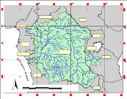
The study area comprises The Congo River Basin, bounded between Latitude 10⁰ and 15⁰S and between longitude 10⁰ and 35⁰ degree East (Figure 1). This area covers several countries in Africa: Democratic Republic of the Congo (DRC), the People's Republic of the Congo, the Central African Republic, and partially through Zambia, Angola, Cameroon, and Tanzania. The Congo River (also known as the Zaire) is over 4,375 km long. It is the fifth-longest river in the world, and the second longest in Africa - second only to the Nile River in North-eastern Africa. The Congo ranges in width from 0.8 to 16 km depending on the location and time of year (The Living Africa, 1998).

N

Cameroon

Congo Rep.

500 0 500 1000 Kilometers

Gabon

Angola

Central Africa

D.R.Congo

Sudan

Rwanda

Uganda

Zambia

Ta

nzania

Figure 1 General Location Map: Position of the study area in Africa

The Congo River forms in the southern-most part of the DRC where the Lualaba and Luvua Rivers meet, then flows to Stanley Falls, near Kisangani, a point just north of the Equator before taking on a counter clockwise course. The Congo loops first to the northeast, then to the west, and then to the south before reaching an outlet into the Atlantic Ocean, feeding a river

basin that covers over 4.1 million km². At the outlet into the Atlantic Ocean, the Congo discharge up to 34,000 m³/s of water per second (The Living Africa, 1998).

Within the Congo's banks can be found over 4,000 islands, more than 50 of which are at least 10 miles (16 km) in length. It is because of these islands that some stretches of the Congo are not navigable. It has been estimated that almost 400 km of the Congo are not navigable due to these islands plus a number of cataracts, in particular at Livingstone Falls.

2.2 Physiography

The Congo basin is the most clearly bounded by various geographic depressions situated between the Sahara to the north, the Atlantic Ocean to the south and west, and the region of the East African lakes to the east (Britanica, 2007). Tributaries flow down slopes that vary from 274.3 m to 457.2 m into a central depression that forms the basin. It measures more than 193 1.2 km north to south (from the Congo-Lake Chad watershed to the Angolan plateaus). West to east - from the Atlantic to the Nile-Congo watershed - it also measures 193 1.2 Km (Butler, 2006).

The Congo basin has a large depression in the central portion. Referred to as a "cuvette", it is a large, shallow, saucer-shaped area. This depression contains Quaternary alluvial deposits which rest on thick sand and sandstone sediment of continental origin. Along the eastern edge of the cuvette outcrops of sandstone are formed. The cuvette has a filling that dates to Precambrian times (570 million years ago). Studies have shown that the sediment has built up over time from the erosion of the formations that surround the cuvette. The Congo River system is composed of three distinct sections - the upper Congo, the middle Congo and the lower Congo.

Kisangani is situated downstream from the Boyoma Falls and is at the beginning of where the Congo River becomes navigable. For 1000 miles (1610 km) the river flows towards Kinshasa. At first the river is narrow but soon widens as it enters the alluvial plain. From the point where the river widens, strings of islands occur which divide the river into different forms. The width of the Congo River can vary from 3.5 miles to 7 miles, reaching up to 8 miles at the mouth of the Mongala River. Along the banks of the river are natural levees which have been formed by deposits of silt. When the river floods these levees are washed away and the river banks increased in width.

The middle Congo is characterized by the narrowing of the river. The banks are a half-mile to a mile apart, the river is much deeper and its current is high. This section of the Congo is referred to as the Chenal (Channel) or Couloir (Corridor). It is along this stretch of the river that its principal tributaries flow into the Congo. They include the Ubangi River, Sangha River and the Kwa River.

This results in a tremendous increase in the flow of water from 7079 m³/s at Kisangani to its maximum when it reaches Kinshasa

NE

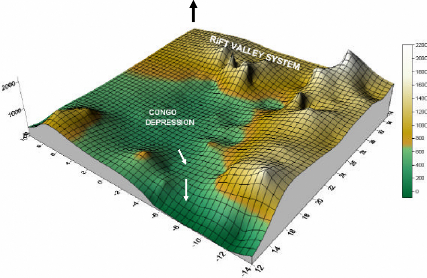
Figure 2 The Congo River Basin Elevation System. The highest station elevation is located in the Tanzanian region while the lowest, at the Atlantic Ocean (Note: this elevation grid is derived from the elevation of the selected 145 meteorological stations falling inside the study area)

From the middle Congo (Chenal) the river divides into two. One branch forms Malebo Pool, which is 24 mile by 27.3 miles large. This is the end of the middle Congo. Just downstream are the first of 30 waterfalls as the river continues to flow towards Matadi. At Matadi, the Congo's estuary begins in a narrow channel only half a mile to a mile wide. Eventually it widens below Boma but islands are once again a factor, dividing the river into several forms. The Congo now flows freely into the Atlantic Ocean.

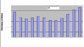
2.3 Hydrology

The Congo has a regular flow, which is fed by rains throughout the year. As recorded at Kinshasa, the flow has for years remained between the high level of 65411.92 m³/s, recorded during the flood of 1908, and the low level of 21407.54 m³/s, recorded in 1905. During the unusual flood of 1962, however, by far the highest for a century, the flow probably exceeded 73623.8 m³/s (Encyclopedia Britannica, 2007). At Kinshasa, the river's regime is characterized by a main maximum at the end of the year and a secondary maximum in May, as well as by a major low level during July and a secondary low level during March and April (Figure 4, Table 1). In reality, the downstream regime of the Congo represents climatic influence extending over 20° of latitude on both sides of the equator, a distance of some 2253km.

The Congo River's flow and water levels are affected by the rains all year round. It is the effects of rainfall throughout the regions whose rivers and tributaries contribute to the Congo River that influence the fluctuations in the flow of the river. However, because the Congo basin has an immense area, the weather pattern in one particular region will not have much effect on the river's overall levels. For example, heavy rainfall in the northern areas that contribute to the

Table 1 River discharge at KINSHASA gauge (after Vorosmarty et al, 1998) Station: Kinshasa, Latitude: 4.3o S/ Longitude: 15.3o E, Elevation: River: Zaire,
Country: Congo D.R., Area: 3475000 km2

-	Jan	Feb	Mar	Apr	May	Jun	Jul	Aug	Sep	Oct	Nov	Dec	Ann
m ^3 /s	47494	37649	34713	37172	39150	36717	31703	31087	36366	43172	51708	56082	40251
mm	36.6	26.4	26.8	27.7	30.2	27.4	24.4	24	27.1	33.3	38.6	43.2	366
km ^3	127	91.9	93	96.3	105	95.2	84.9	83.3	94.3	116	134	150	1270
l/s/km ^2	13.7	10.8	9.99	10.7	11.3	10.6	9.12	8.95	10.5	12.4	14.9	16.1	11.6
%	9.83	7.79	7.19	7.7	8.11	7.6	6.56	6.44	7.53	8.94	10.7	11.6	100

40000

60000

20000

50000

30000

10000

0

Jan Feb Mar Apr May Jun Jul Aug Sep Oct Nov Dec

Month

Mean Discharge Regime (1903-1983)

Discharge

Figure 3 Mean Discharge Regime of the Congo River Basin at the Kinshasa gauge

40000

20000

80000

60000

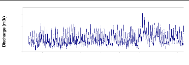
Jan-00 Jan-10 Jan-20 Jan-30 Jan-40 Jan-50 Jan-60 Jan-70 Jan-80

Time

Monthly Discharge at Kinshasa gauge (Mean 1903-1 983)

Figure 4 Monthly discharge of the Congo River (Kinshasa gauge). Mean 1960-1990

Patterns have been established in the past and the river can be expected to have higher levels
in December and May due to the rainy season. The levels are expected to be low in March and

April and even lower in July in response to the dry season. If some of the weather patterns change drastically, resulting in floodwaters arriving at the same or different times, then the anticipated water levels are affected accordingly.

2.4 Climate

The Congo basin is located in the equatorial belt. This location ensures that different parts of the Congo basin receive substantial rainfall throughout the year; with a decreasing trend of rainfall with latitude. The northern and central portions of the basin have two major rainfall seasons which begin in March and October each year (Kazadi, 1996). The northernmost points of the basin, situated in the Central African Republic, receive 8 to 406.4 mm during the course of a year, which is less than the average near the equator; the dry season, however, lasts for four or five months, and there is only one annual rainfall maximum, which occurs in summer.

In the south, the two rainfall seasons gradually merge into a single season beginning in December and lasting for six months each year. In the far southern part of the basin -- at a latitude of 12° S, in the Katanga region -- the climate becomes definitely Sudanic in character, with marked dry and wet seasons of approximately equal length and with mean rainfall of about 1245 mm a year.

The rainfall peaks are associated with the passage of the Inter-Tropical Convergence Zone (ITCZ), which is a large zone of low pressure caused by excessive heating from an overhead sun. During the northern summer, the midday sun is directly overhead in the tropical regions of the Northern Hemisphere. This results in higher temperatures and consequently, lower air pressures at the surface. Moist air flows from the oceans towards these low pressure areas. The moisture is released as rainfall on the land surface when the air is forced to rise on entering the convergence zone or by orographic effects. The ITCZ causes heavy rainfall in the areas it passes over as it moves north and south between the tropics during the respect northern and southern summers. The Congo basin is thus representative of a large river basin in which the spatial distribution of input varies significantly with time.

Figures 6 bellow shows the monthly distribution of rainfall, Evapotranspiration and temperature for 8 stations over the Conog Basin. Figure 7 and Table 2 give the evective rainfall for three virtual stations located in the southern hemisphere, northern and the center of the basin.

Figure 5 Meteorological profile of D.R.Congo

Table 2 Effective Rainfall distribution in the Congo Basin

Long	Lat	Dec	Jan	Feb	Mar	Apr	May	Jun	Jul	Aug	Sep	Oct	Nov
12	-14	32	30.1	40.4	75.6	44.6	1.8	-0.5	-1.2	-2.8	-5.1	0.7	32
23.58	-2	131.3	113.6	104.2	129.9	126.3	106	57.1	61.7	99.4	137.6	139.2	131.3
35	10	5.8	11.9	12.7	43.5	92.7	114.8	84.7	115.5	129.8	121.1	98.7	5.8

160

140

120

100

-20

40

80

60

20

0

Lowest station Center Upper Station

Grid: Long. 23.58, Lat. -2.00

Months

Figure 6 Long-term monthly average of Effective Rainfall (1961-1990) at grid cell.

Figure 7 Effective rainfall distribution for three selected grids in the Area

2.5 Soils

Generally, there are two types of soils in the study area: those of the equatorial areas and those of the drier savanna (grassland) regions. The equatorial soils occur in the warm, humid lowlands of the central basin, which receive abundant rainfall throughout the year and are covered mainly with thick forests. This soil is almost fixed in place because of the lack of erosive forces in the forests. In the shore areas, however, swamp vegetation has built up a remarkably thick soil that is constantly nourished by humus, the organic material resulting from the decomposition of plant or animal matter. Although in the savanna regions the soils are constantly endangered by erosion, the river valleys contain rich and fertile alluvial soils. Special note should be made of the highlands of eastern Congo in the Great Lakes region, which are partly covered with volcanic lava that has been transformed into exceptionally rich soil.

An agronomic soil map at 10X10 spatial resolutions (Figure 1 1) is available at FAO-UNESCO database (1984). This map can be resampled and reclassified according to the objectives of the research. In Hydrological modelling, a textural Soil map is required to derive soil retention properties such as field capacity, wilting point, available water content, etc. For the southern Africa, Alemaw and Chaoka (2003) demonstrate the usefulness of the agronomic soil data in deriving soil texture classes for hydrological modelling.

2.6 Land cover/use and Population density

The land cover pattern of the Congo basin is viewed in Figure9 and summarised in Table 3. Mostly, the basin is coverd by green and dense forest. Dryer regions occupy less then 0.2 % of the basin. Figure 10 below shows the population density distribution over the basin.

Figure 8 Congo Basin Agronomic Soils Map. The polygon limit the Congo watershed
Table 3 Land cover distribution in the Congo River basin (after World river resources, 2003)

Percent Forest cover	44.0
Percent Grassland, Savanna and Shrubland	45.4
Percent Croplands	7.2
Percent Irrigated Cropland	0.0
Percent Dryland Area	0.2
Percent Urban and Industrial Area	0.2

Figure 9 Vegetation and Land cover and uses over the Congo River Watershed (after World river resources, 2003)

Figure 10 Population density distribution over the Congo River Watershed: Basin area 3,730,881 sq.Km, Average Population Density (people per sq.km): 15, Number of large cities (100,000 people).

2.7 Geology

The Geology of the Democratic Republic of Congo is characterized by two large structural units separated by discordance and/or a significant gap: The Formations of covers (Phanerozoic), not metamorphosed, generally fossiliferous, and of age ranging between the Upper carboniferous and the Holocene; and the Basement terrains (Precambrian shield): Highly metamorphosed + shielded contouring continuously the basin.

2.7.1 Basement formation

The Basement terrains are subdivided in "tectostratigraphic" units:

a) Archean shields of age equal to or higher than 2500 MA levelling to the northern Congo and Kasaï;

b) Lower and middle Precambrian Belts (2.500 to 1.300 MA) whose sediments settled in meridian mobile zones located on the Eastern and Western edges of the Craton and in the intra - cratonic valleys;

c) Upper Precambrian called Katangien whose sediments settled on the epicontinental platforms and in the «subsiding surfaces» of the craton of Congo (Katanga folded and tabular).

2.7.2 Surface formations

The surface formations are grouped into four zones as follows:

(i) A littoral zone, ranging between the Atlantic Ocean and the Mayumbe mounts (Crystal Mounts);marine formations tertiary and Cretacic age are well developed there;

(ii) The central basin where the deposits of Mezoic and Cenozoic ages spread out; vast terrains level on the circumference of the Basin;

(iii) The edge of old grounds subdivided in six unconnected areas ;

(iv) The tectonic valley of the East of Congo occupied by particular Cenozoic formations and characterized by recent volcanic activities.

The formations of each one of these 4 great zones are covered indifferently by recent formations, the ochre series of sands and the series of the polymorphic sandstones.

CHAPTER THREE

3.0 LITERATURE REVIEW

3.1 Hydrological models

Hydrological model have been largely detailed and classified (Figure 1) based on multiple parameters such as the model input data sets types, and the physical characteristic of the model among others. However, Hydrological models have, traditionally, been modelled as physically-based or conceptual depending on the complexity and extent of completeness of the structure of the model (Beven, 1989; Refsgaard et al., 1989; Bergstrom, 1990; Refsgaard, 1996, 1998).

Hydrological
Models

Deterministic

Stochastic

Grid based

Subwatershed

No Distribution

Figure 11 Hydrological Model Classification

Probabilistic

Time Series

Physical
Based

Distributed

Conceptual

Lumped

Empirical

In physically-based water balance models, all the physical phenomena like precipitation, evapotranspiration, ground water inflow, ground water outflow and storage need to be quantified and modelled. Models are further classified into lumped or distributed, based on basin terrain (Bergstrom and Graham, 1998). In lumped models, spatial variability in hydrologic parameters or meteorological related data are not accounted for, meaning that they are averaged or assumed uniform over the system, whereas, in distributed models spatial variability is explicitly accounted for by assuming uniformity over smaller modelling units by sub dividing the bigger system based on physical properties. In most of the distributed hydrologic models, these units are delineated by combining climatic components, topography, soil properties, land use properties and other pertinent properties. Distributed models are especially useful, for example, when impacts of land use change are to be studied or for analyzing spatially varying flood responses (Koka,

2004). The Lumped models are easy to implement, but do not account for terrain variability whereas Spatially-distributed models require sophisticated tools to implement, and account for terrain variability (Oliveira, 2002).

A statistical model derives an empirical relationship between precipitation, infiltration, flow and any other parameters that are included in the model. The relationship is derived based on observed data for all the dependent and independent parameters in the model. The best relationship is identified using suitable statistical parameters (Sukheswalla, 2003).

Large scale modeling of streamflow can be done efficiently using simple models (Becker and Braun, 1999; and Wolock and McCabe, 1999). Distributed models require high resolutions for efficient modeling like the MIKE SHE model (Ewen et al., 1999) and the TOPMODEL (Beven et al., 1994). However, for large scales such high resolution is not always available. Also, distributed models are generally not practical and efficient for large-scale modelling (Becker and Braun., 1999), while statistical lumped models that fulfil large scale modelling requirements of resolution and computation time are better (Becker and Pfützner, 1987).

Using the cell-to-cell model, a watershed can be represented as a single cell, a cascade of n equal cells, or a network of n equal cells (Singh, 1989). The storage in the cells is calculated as given below:

(1)

dS= -

dt

^t I O

t t

where, S_t is the time-variant storage in a grid cell,

I_t is the summation of input coming into the cell from

upstream cells and the runoff generated in the cell, and

Q_t is the outflow from the cell which is calculated by

various methods, e.g. the linear reservoir method.

Equation (1) is a generalized water balance model which can be applied in different situations: atmospheric, surface, soil-water, groundwater models. The types of input variables are defined by the researcher according to the problem. Several books, papers ad reports describing the application of equation (1) are available, viz Thornthwaite and Mather (1957), Chow et al (1988), Reed et al (1997) and Rasmusson (1997).

3.2 Water Balance Model approaches

In order to understand water balances, complex hydrologic systems have always been simplified. Thornthwaite and Mather (1957) conceptualized a Catchment water balance model for long term monthly climatic conditions; which then led to many researches on water balance models for similar conditions on a catchment, region or a continent. Typical examples for these models are the GIS-based water balance model for the Southern Africa of Alemaw and Chaoka (2003), the Grid-based model for Latin America of Vorosmarty et al. (1989), Reed et al. (1998), the Grid -based model for Amazone

basin of Marengo (2005), the Rhine flow model of Van Deursch and Kwadijk (1993); and the Large-scale water balance model for the upper Blue Nile in Ethiopia of Conway (1997), and the spatial water balance of Texas (Reed et al., 1998).

Hydrological water balance models can be based on the interactions between the water, atmosphere, and land surface; which is a combination of the atmospheric water balance, Surface Water Balance and the soil Water Balance Studies.

3.2.1 Atmospheric Water Balance Studies

The estimation of hydrologic flux using Atmospheric water balance has been studied by a number of researchers (Reed et al., 1998; Rasmusson, 1967; Brubaker et al., 1994; and Oki et al., 1995; Marengo, 2005), among them. Rasmusson (1967), Brubaker et al. (1994) and Oki et al. (1995) describe atmospheric water balance at river basin, continental, and global scales. Rasmusson (1967) analyzes the characteristics of total water vapor flux fields over North America and the Central American Sea. Reed et al (1998) presents the atmospheric water balance of Texas and Marengo (2005), that of the Amazone basin.

The atmospheric branch of the water balance has always been expressed in the form of a

simple equation of vertically integrated terms: Q

(2)

dW Q P E

r

= -?× - +

t

d

where -?×Q=C	expresses the vertically integrated moisture convergence, Q is the

water-vapor fluxe, P is the precipitation, E is the Evapotranspiration, and dW/dt represents the atmospheric storage (water vapour) change term which is generally negligible for averages over a month or more (Roads et al., 1994; Eltahir and Bras, 1994; Reed et al., 1998; Curtis and Hastenrath, 1999; Costa and Foley, 1999; Zeng, 1999, Marengo, 2005). Given adequate data, the atmospheric water balance is a promising method for estimating regional evaporation, runoff, and changes in basin storage (Reed et al, 1998).

Although the atmospheric water balance model is efficient to estimate hydrologic flux within an area, significant uncertainties in runoff estimation using atmospheric data exist even at the continental scale (Reed et al., 1998). Comparing their estimated continental runoff with those given by Baumgartner and Reichel (1975) in North America river runoff, Brubaker et al. (1994) and Oki et al. (1995) note the fact that poorly defined continental or basin boundaries may contribute to inaccuracies in runoff estimation. To obtain an accurate runoff form vertically integrated vapour flux convergence, the annual change in atmospheric water storage and surface water storage should be negligible (Reed et al, 1998).

3.2.2 Soil Water Balance Studies

The simple bucket models have been developed by hydrologist to simulate near-surface
hydrological model in the conditions where detailed data about soil layers, depth to

groundwater, and vegetation are not available (Reed et al, 1998). Despite numerous uncertainties associated with the simple soil-water budget model many researchers have applied this type of model to problems ranging from catchment scale studies to the global water balance and climate change scenarios (Thornthwaite, 1948; Thornwaite and Mather, 1957; Manabe, 1969; Mather, 1978; Dunne and Leopold, 1978, Shiklomanov, 1983; Alley, 1984; Willmott et al., 1985; Mintz and Serafini, 1992; Mintz and Walker, 1993, Alemaw and Chaoka, 2003, Sen and Ambro Gieske, 2005, Marengo, 2005).

The "bucket" model approach is attractive because of its simplicity and requires minimal input data: precipitation, potential evapotranspiration, and soil-water holding capacity (Reed et al, 1998). The studies by Willmott et al. (1985), Mintz and Walker (1993), and Mintz and Serafini (1992), are climatology studies that present the global distributions of precipitation, evapotranspiration, and soil moisture. Mintz and Serafini (1992) compare their evapotranspiration estimates for sixteen major river basins throughout the world with those derived from river runoff analysis made by Baumgartner and Reichel (1975) and the values show reasonable agreement (Reed et al, 1998).

At a smaller scale, Mather (1978), quoted by Reed et al (1998), describes the application of a soil-water budget model to several watersheds in the coastal plains of Delaware, Maryland, and Virginia. Comparisons between measured and computed runoff values are rather poor for monthly data, but better for annual data.

In its simplest form, the soil-water budget model does not account for situations where the precipitation rate is greater than the infiltration capacity of the soil. Mather (1978) describes one approach to remedy this problem, that is, to first use the SCS method to estimate direct overland runoff and substract this amount from the precipitation before it is allowed to enter the soil "bucket." This approach appears to yield better results. A similar approach of taking an initial rainfall abstraction before allowing precipitation to enter the soil column for climatological budgeting was used in a study of the Niger Basin (Maidment et al., 1996), in southern Africa region (Alemaw and Chaoka, 2003) and in the Limpopo basin (Alemaw, 2006).

3.2.3 Surface Water Balance Studies 3.2.3.1 Water Balances

The commonly used method in hydrologic studies, namely the surface water balance, relies on the fact that with the exception of coastal areas, the landscape can often be divided into watershed units from which there is only one surface water outflow point (Reed et al, 1998). If assumed that change in storage is negligible and that there are no significant inter-watershed transfers via groundwater or man-made conveyance structures, providing that the average watershed precipitation and runoff can be measured with reasonable accuracy, the annual evaporative losses from a watershed can be estimated by Empirical relationships which are often used to estimate mean annual or mean monthly flows in ungaged areas; this approach is used in this study (Reed et al, 1998).

3.2.3.2 Runoff Mapping

Arnell (1995), Lullwitz and Helbig (1995), Reed et al (1998), Alemaw and Chaoka (2003) and Alemaw (2006) describe studies of runoff mapping using a geographic information system (GIS) to manage spatial data at a regional or continental scale.

Arnell (1995) presents five approaches for deriving gridded runoff maps at a 0.5 degree grid resolution; they include: (1) simply averaging the runoff from all stations within each grid cell, (2) statistically interpolating runoff between gages, (3) using an empirical relationship that relates runoff to precipitation, potential evaporation, and temperature, (4) using a soil-water balance type model, and (5) overlaying grid cells onto catchment runoff maps to derive area-weighted runoff estimates. In a study using the 5 approaches to map runoff over a large portion of Western Europe, the results show that method (5) produces the most reasonable estimates. In a study similar to that of Arnell (1995), Lullwitz and Helbig (1995) created 0.5⁰ grid runoff maps for the Weser River in Germany. In both this papers, authors noted that 0.5 degree runoff maps can be useful for validating general circulation models (GCM's). Church et al. (1995), using an interpolation method to create runoff maps, present maps of evapotranspiration (ET) and runoff/precipitation (R/P) ratios for the northeastern United States. A different approach of mapping surface runoff, similar to Arnell's method (Arnell, 1995), combining an empirical rainfall-runoff relationship and watershed runoff balancing was used by Reed et al (1998).

Alemaw and Chaoka (2003) developed a GIS based hydrological model simulating the spatial and temporal distribution of water budget parameters for the Southern Africa region. This model was slightly modified and used for the Limpopo basin (Alemaw, 2006), where monthly runoff is generated from matrix of specific geo-referenced grids.

3.3 Potential evapotranspiration (ETp) and Effective rainfall determination

Potential runoff is defined the maximum possible rate at which evapotranspiration would occur from a large area completely and uniformly covered with growing vegetation which is not short of water under given atmospheric conditions (Weligepolage, 2005).

3.3.1 Estimation of Potential Evapotranspiration

A Number of approaches have been developed for estimating the ETp or ETref based on different theoretical concepts. Most commonly applied methods for hydrological studies can be classified into four categories on the basis of their data requirement (Weligepolage, 2005):

a) Temperature based methods- use only daily average air temperature and some times the day length.

b) Radiation based methods- use both the net radiation and air temperature data for estimating ET.

c) Combination- use net radiation, air temperature, wind speed and relative humidity data based on the Penman-Monteith combination equation.

d) Pan measurement- use pan evaporation with modifications depending on wind speed, temperature and humidity.

The methods that do not require information about the nature of the surface, estimate the reference crop evapotranspiration rate where as others are surface specific and do require information about albedo, vegetation height, maximum stomatal conductance, leaf area index and other factors.

The American Society of Civil Engineering (ASCE) and Consortium of European Research Institutes have undertaken major studies to evaluate the performance of different evapotranspiration estimation procedures under different climatologic conditions. Both have indicated that the FAO Penman-Monteith approach of reference crop evapotranspiration as relatively accurate and consistent performance in evapotranspiration estimation (Allen et al, 1998).

The following paragraph gives details on the Penman-Montheith method where the Potential evapotranspiration is considered to be the Reference evapotranspiration:

ET=

⁰ Ä + +

(1 0 . 34 )

U 2

(3)

900

0. 40 8Ä

+

+

( )

R G

-

n

U e

2 ( a

- e_d)

T

273

where; ETo =
Rn	=
G	=
T	=
U2	=

Reference crop evapotranspiration (mm/day) Net radiation at crop surface (MJ m^-2 d^-1) Roil heat flux (MJ m^-2 d^-1)

Average temperature (^oC)

Windspeed measured at 2m height (m s^-1) (e_a-ed) = Vapour pressure deficit (kpa)

=? Slope vapour pressure curve (kPa ^oC^-1)

? = Psychometric constant (kPa ^oC^-1) 900 = Conversion factor

3.3.1.1 Net radiation

The Net radiation is s determined as follows;

R _n =R _ns -R nl (4)

n

R = 0 .77(0 .25 + 0 . 5 ) (5)

ns Ra

N

(6)

n

nl 2.45.10 (0.9 0.1)(0.34 0.14 )( )

= + - +

⁹ ed T T

4 4

R kx kn

N

G = 0.14(Tmonthn - T monthn-1) (7)

where; R_n = net radiation

Rns = net short wave radiation (MJ _m-2 _d-1)

Rnl = net longwave radiation (MJ _m-2 _d-1)

n /N = relative sunshine fraction

Tkx = maximum temperature (K)

Tkn = minimum temperature (K)

ed = actual vapour pressure (kPa)

G = soil heat flux (MJ _m-2 _d- 1₎

Tmonth n = mean temperature in month n (^oC)

Tmonth n-1 = mean temperature in preceding month n-1 (^oC)

3.3.1.2 Mean Relative Humidity

The humidity expressed as saturation vapour pressure at dewpoint temperature (mbar) has been converted to mean daily relative humidity from maximum and minimum temperatures according to the following relationship:

RH RH

+ ?

RH e

= =

max min

min 2 d ? ?

50 50

+ (8)

e e ?

a Tmean a T

( ) ( max) ?

Where ed = saturation vapour pressure at dewpoint temperature (kPa) ea = saturation vapour pressure at minimum temperature ea(Tmax) = saturation vapour pressure at maximum temperature The saturation vapour pressure is determined according to Teten's formula: e a 0.611exp ( 17.27 T T 237.3 ) = +

(9)

Where e_a = saturation vapour pressure at temperature T (^oc) 3.3.1.3 Wind speed

The original wind data expressed in m/s are convereted into km/day according to:

U2=U ₂ ×86.4 (10)

*

Where; U₂ = wind speed in km/day at 2 m height

U₂ = wind speed in m/s

*

3.3.1.4 Solar radiation

As no measured data on solar radiation are available, solar radiation has been estimated from measured sunshine hours according to the following relationships:

n R ) p = (0 .25 + 0 . 5 ^s 100

R (11) a

Where; R_s = solar radiation (MJ m^-2d^-1)

R_a = extraterrestrial radiation (MJ m^-2d^-1)

0.25, 0.5 = Angstrom coefficients

n

n = (12)

* 100

^p N

Where; n = daily sunshine hours (hr)

np = daily sunshine percentage (percentage.)

N = day length (hours), depending on latitude and month of the year.

From the computed ET_o series, the 20% exceedence probability (1 in 5 years-return period) values are estimated.

3.3.2 Estimation of Effective Rainfall

Effective rainfall is defined as that part of the precipitation which is effectively used for evapotranspiration by the crop. Four methodologies are given below to determine the effective rainfall:

a) Fixed percentage rainfall: effective rainfall is calculated according to:

EPPT=a×PPT (13) Where a, is a fixed percentage to be given by the user to account for losses from runoff and deep percolation. Normally losses are around 10 to 30%, thus a = 0.7- 0.9, EPPT is the effective precipitation and PPT, the total precipitation

b) Dependable rain: based on an analysis carried out for different arid and subhumid climates an empirical formula was developed in FAO/AGLW to estimate dependable rainfall, the combined effect of dependable rainfall (80% prob.exc.) and estimated losses due to runoff and percolation. This formula may be used for design purposes where 80% probability of exceedance is required. Calculation according to:

EPPT=0.6PPT-10; forPPT<70mm (14)

EPPT = 0.8PPT - 24; for PPT > 70mm (15)

c) Empirical formula: The parameters may be determined from an analysis of local climatic records. An analysis of local climatic records may allow an estimation of effective rainfall. The relationship can, in most cases, be simplified by the following equations:

EPPT= aPPT-b; forPPT<Z(mm) (16)

EPPT=cPPT+d; forPPT>Z(mm) (17)

Values for a, b, c and z are correlation coefficients.

d) USDA Soil Conservation Service Method: is a method where monthly effective rainfall (in millimetre) can be calculated from monthly total rainfall (in millimetre) according to the following equations (18, 19); this mwthod is adopted whenever daily rainfall data are not available.

EPPT = PPT(125 - 0.2PPT)/125; for PPT 250 mm

< (18)

EPPT = 125 + 0.1PPT; forPPT > 250mm (19) The use of these methods depends on the time scale of the model and the availability of data.

CHAPTER FOUR

4.0 METHODOLOGY

The present chapter comprises two major sections describing the watershed and streams characteristics method of determination and the water balance modelling method.

4.1 Watershed and streams characteristics

The concept of a watershed is basic to all hydrologic designs. Watershed has been defined as an area of land draining into a stream at a given location (Chow et al, 1988). In other words and usually a watershed is defined as the area that appears, on the basis of topography, to contribute all the water that passes through a given cross section of a stream. The surface trace of the boundary that delimits a watershed is called a divide, and the horizontal projection of the area of a watershed is called the drainage area of a stream at that cross section, while the location of the stream cross section that defines the watershed is determined by the analysis.

Since large watersheds are made up of many smaller watersheds, it is necessary to define the watershed in terms of a point. This point is usually the location at which the design is being made and is referred to as the watershed «outlet». With respect to the outlet, the watershed consists of all land area that «sheds» water to the outlet during a rainstorm. Using the concept that «water runs downhill», a watershed is defined by all points enclosed within an area from which rain falling at these points will contribute water to the outlet (McCuen, 2005).

To delineate the Congo River Watershed and streams network, a Digital Elevation Model (DEM), HYDRO 1K with 1 km of spatial resolution, later on described, was used and processed with Geographical Information System packages viz Integrated Land and Water System (ILWIS) and ArcGIS.

In the following section are presented different steps followed for the DEM-Hydro watershed processing. The purpose of this chapter is to define and hydrogeomorphologically charcterise the watershed and streams behaviours of the Congo basin, availing useful data sets for hydrological modellings.

4.2 Watershed and drainage network Processing Method

The detailed processing method presented bellow (Figure 12) is a combination of techniques used in GIS ILWIS 3.4, ArcINFO 9.2 and ArcView 3.2 packages; it consists in:

1 DEM visualization

2 Flow Determination (Fill sinks, Flow direction, Flow accumulation, Flow

Modification)

3 Variable threshold computation

4 Network and Catchment Extraction (Drainage network extraction, Drainage

network ordering, Catchment extraction, Catchment merge

5 Compound Parameter Extraction (Overland flow length, Compound Index

calculation)

6 Statistical Parameter Extraction (Horton statistics, aggregate statistics, cumulative

hypsometric curve, class coverage).

DEM
1 kHYDRO 30sec

Statatistical Parameters Extraction

HORTON statistics

Cumulative Hypsometric Curve

Threshold

Outlets coordinate

Digitized Drainage

Minimum Drainage Length

Compound Parameters Extraction

Drainage Network Ordering

Catchment Extraction

Catchment Merge

Drainage Network Extraction

DEM Optm

DEM Fill Sinks

Flow Direc

Flow Accu

Drainage Network Ordering Map

DEM Optm Map

DEM Filled Map

Flow Direct Map

Flow Accu Map

Drainage Map

Overland Flow length Map

Catchment Maps

Extract Stream Segments + Attributes

Wetness/Power/Sediment indexes Maps

Catchment Merged Map

Longest Flow Path Segment Map

Figure 12 DEM Processing flow chart: Extraction of Drainage network, Catchment and Horton Parameters.

4.3 DEM-Hydro processing output maps

This section presents and describes the findings of the DEM-Hydro processing technique accordingly to their application in hydrological modelling.

4.3.1 DEM Visualization and areal distribution over elevation

The topography is mostly characterised by a more or less flat are in the centre of the study area (Figure 14). This area is called «Central cuvette» and is limited by the Great Rift Valley to the East, mountainous regions in the north-western and south-eastern corner of the study area.

The altitude varies between -99999 and 4657 m with an average of 1886 m. In HYDRO1k DEM, pixels with missing data are assigned a negative value of -99999. Extracting the area covering exclusively the Congo Watershed, the elevation mean is around 238 m aswl with a minimum of 0 m.

2500

2000

1500

1000

500

0

1 1

26 24

12

Elevation ranges

27

3 0 000 0

% of Elevation Area

40

80

60

20

0

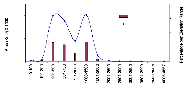
Figure 13 Areal distribution at different altitude (The area in a logarithmic scale)

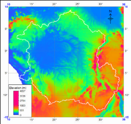
Figure 14 DEM visualization map for Cental Africa. The defined colored polygone delineated the Congo River basin.

Table 4 Summarised Statistics for the DEM

Elevation	npix	npixpct	npixcum	npcumpct	Area (Km square)
0-100	46440	0.65	41461805	553	46956
101-200	88017	1.24	47682206	636	88994
201-500	1984879	27.92	342086982	4563	2006916
501-750	1770620	24.91	869454897	11598	1788574
751-1000	901295	12.68	1183992072	15794	911302
1000-1500	2006891	28.23	3176337475	42371	2029172
1501-2000	274325	3.86	3693851852	49274	277371
2001-2500	28808	0.41	3738833270	49874	29128
2501-3000	6081	0.09	3716166768	49572	6149
3001-3500	1168	0.02	2840777253	37895	1181
3501-3999	467	0.01	1866541342	24899	472
4000-4005	n/a	0.00	-	-
4006-4657	114	0.00	607211659	8100	115

PS: npix= number of pixels, npixpct= percentage of number of pixels, Npicum = cumulated percentage of number of pixels. In colone 2, the pixel numbers with -9999 elevation value are ignored.

4.3.2 Flow direction map

This step comes after fill-sink step. The filled DEM was then used to find the flow direction map using standard D-8 algorithm (Figure 15). Flow direction is calculated for every central pixel of input blocks of 3 by 3 pixels, each time comparing the value of the central pixel with the value of its 8 neighbors. The steepest slope method was used for this study to find the steepest downhill slope of a central pixel to one of its 8 neighbour pixels and assign to flow directions.

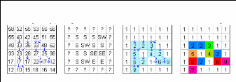
Calculating flow directions from a DEM (steepest slope)

Output flow direction map

Calculating flow accumulation

Output flow accumulation map

Figure 15 D-8 algorithm: Based on the output Flow direction map, the Flow accumulation operation counts the total number of pixels that will drain into outlets (after ILWIS 3.4 Manual)

The output map shown in Figure 16 contains flow directions grids as N (to the North), NW (to the North West), NE (to the North East), SE (to the South East), S (to the South) and SW (to the South West).

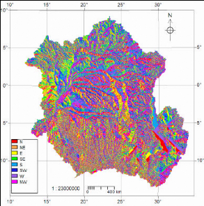
Figure 16 Flow direction map

The histograms (Figure 17) indicate that the flow direction algorithm tends to favor the cardinal directions (north, south, east and west) over the diagonal directions (northeast, northwest, southeast and southwest). For the entire dataset (rectangular area) 63 % of grids cells had flown in a cardinal direction as compared to 37 % diagonals. This indicates that the flow direction algorithm used in the model is predisposed in favor of flow through the cardinal directions. The same observation was done in previous study on the basin (Kwabena, 2000).

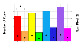
600000

400000

200000

700000

500000

300000

N NE E SE S SW W NW

Flow Direction Orientation

CB_Fdir_filled x Number Pixel Perc CB_Fdirjilled x NPix

60

40

20

80

0

100

Figure 17 Histogram of Flow Direction for Central Africa

Table 5 Summarised statistics for the Flow direction grid map in the area of study.

Flow direction Orientation	Number Pixel	% Number pixels	Area (Km2)
E	579477	15	579477
N	536518	14	536518
NE	334119	9	334119
NW	372838	10	372838
S	600426	16	600426
SE	314363	8	314363
SW	382729	10	382729
W	658407	17	658407
Min	314363	8.3	314363
Sum	3778877	100.0	3778877

4.3.3 Flow accumulation

The flow direction grid developed at the previous step is then used as input data for Flow Accumulation grid calculations. The flow accumulation map contains cumulative hydrologic flow values that represent the number of input pixels which contribute any water to any outlets; the outlets of the largest streams (drain, river) will have the largest values which is 3778906 for the Congo River basin. The grid generated (Figure 18) has a minimum of 1 and a maximum of 3778906 pixels values for computed flow accumulation matrix.

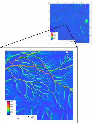
Figure 18 Flow Accumulation map; on top: Entire basin, on bottom: A selected area

4.3.4 Drainage network extraction and ordering

The Drainage Network Extraction operation extracts a basic drainage network (raster map). As input it is required the output raster map of the Flow Accumulation operation and a defined threshold value. A threshold value, i.e. a value for the minimum number of pixels that are supposed to drain into a pixel to let this pixel remain as a drainage in the output map; the larger is this value, the fewer drainages will remain in the output map. Depending on the flow accumulation value for a pixel and the threshold value for this pixel, it is decided whether true or false should be assigned to the output pixel. If the flow accumulation value of a pixel exceeds the threshold value, the output pixel value will be true; else, false is assigned. A threshold value of 1000 (number of pixels) is used in this process and 1752 stream segments are identified in the Congo River Basin masked (Figure 19).

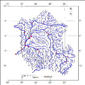
Figure 19 Stream network map masked by the boundary of the Congo River Basin 4.3.5 Catchment and Sub-Catchments extraction

During the Catchment extraction operation, 3435 sub-catchments were extracted. Using the Cross operation 1752 sub-catchements only (Figure 20) were selected; each of them corresponding to a single stream segment from the Drainage network ordering operation. This operation delivers an output raster map, an output polygon map and an output attribute table.

The attribute table (appendix 6) andd Table 6 summarises information for each catchment, such as the area, longest flow path, density, and perimeter of catchment, the total upstream area. Figures 21-22 show 5 sub-catchments corresponding to 5 defined outlets namely Sangha, Ubangi, Kasai and Lualaba. The Congo sub-catchment is generated with the residual area.

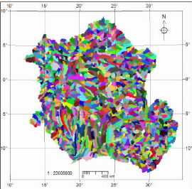
Figure 20 Extracted sub-catchment map in the Congo Basin

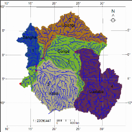
Figure 21 Merged sub-watershed with stream network and majors outlet of the CRB

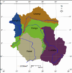
Figure 22 Longest flow path map overlayed on the sub-watersheds of the CRB

4.3.6 Overland Flow map

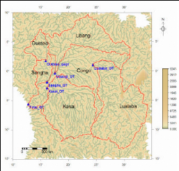
Figure 23 Overland flow distribution in the study area

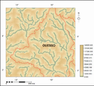
Figure 24 Overland flow distribution in the Ouesso sub-watershed

4.4 Watershed characteristics

Watershed characteristics are subdivided in 2 major groups: physiographical and hydrological. The physiographical characteristics of a watershed influence to a large degree its hydrological responses and especially the flow regime during floods and periods of drought, hence the discharge, and the concentration time, which characterizes the speed and intensity of the watershed's reaction to stress (rainfall), is influenced by the different morphological characteristics. The analysis of the hydrologic behavior of a watershed is done in order to study the hydrologic reaction of the watershed in relation to rainfall. The Horton morphometric parameters will be described separately.

4.4.1 Watershed Geomorphology 4.4.1.1 Area and length

The drainage area (A) is probably the single most important watershed characteristic for hydrologic design and reflects the volume of water that can be generated from rainfall. It is common in hydrologic design to assume a constant depth of rainfall occurring uniformly over the watershed. Under this assumption, the volume of water available for runoff would be the product of rainfall depth and the drainage area. Thus the drainage area is required as input to models ranging from simple linear prediction equations to complex computer models (McCuen, 2005).

The computed watershed area is of 3778879 km², which is strongly closer to 3,780,000km², value estimated by Asante (2000) using ArcMap.

Table 6 Sub-wateshed characteristics of the CRB

1	Ouesso	2364.2	155408	3572.4	22.73	792.9	730197.6	341	762	702
2	Sangha South	2186.6	130671	3117.0	23.59	697.8	625778.7	234	457	343
3	Ubangi	6845.5	639564	15455.1	23.9	2538.5	2472266	291	1272	1133
4	Kasai	5516.5	895179	25007.0	27.62	2102.4	2022944	234	1481	1282
5	Lualaba	7264.1	1109014	27362.9	24.4	3083.4	3020203	429	1842	1446
6	Congo	11000.0	849063	19436.5	22.64	3515.9	3470018	0	1128	1032
	CRB	13475054	3778879	93953.5	24.6	5112.7	5049.5	0	1842	1446

Table 7 Extracted sub-watersheds areas of the CRB

ID	Names	Area (km square)
		Calculated	Repported	Source
1	Ouesso	155408	180418
2	Sangha South	130671
3	Ubangi	639564	613202
4	Kasai	895179	925172
5	Lualaba	1109014
6	Congo	849063
Min		130671
Avg		629817
Sum		3778879	3755441	Asante (2000)

For a better and easier use of the DEM in the Congo River hydrological model, the Congo Basin was subdivided in 6 major sub-watersheds, namely: LUALABA, OUESSO, UBANGI, CONGO, SANGHA SOUTH and KASAI (Figure 22). The Congo sub-watershed is a shapeless basin since it is a residue after the selection of the other 5 major sub-watersheds; therefore it will not be considered in the water balance process.

4.4.1.2 Watershed Shape

The shape of a watershed influences the shape of its characteristic hydrograph. For example, a long shape watershed generates, for the same rainfall, a lower outlet flow, as the concentration time is higher.

A watershed having a fan-shape presents a lower concentration time, and it generates higher flow.

Different geomorphologic indices can be used for the analysis of a watershed if its shape is taken into consideration. The most frequently used index is the Gravelius's index KG, which is defined as the relation between the perimeter of the watershed and that of a circle having a surface equal to that of a watershed.

(20)

P P

K =

G

0.28

2 · A A

Where KG is the Gravelius's shape index, A is the watershed area [km²] and P, watershed perimeter [km].

Musy (2001) presented different values of the Gravelius's index whose comparison to the Congo Basin (Gravelius index = 1.93) makes it to be treated like a circular basin. However, the Gravelius Index varies from one sub-watershed to an other one.

4.4.2 Morphometric Analysis

The morphometric network is defined as the sum of all the watercourses, natural or artificial, permanent or temporary, which contribute to the runoff. The characteristics of a hydrographic network of a watershed are influenced by four main factors: geology, climate, relief and environment.

4.4.2.1 Morphometric network topology

The classification of the watercourses was introduced by Strahler (1957). The order of the watercourses reflects the degree of ramification of the morphometric network from upstream to downstream and it is based on the following principles: (Musy, 2001)

all watercourses without tributaries are of 1 st order;

the watercourse formed by the confluence of two watercourses of different order is going to keep the highest order of the two;

the watercourse formed by the confluence of two watercourses of same order is going to have an order higher with one than the other two.

Seven Sthraler orders and 898 Shreve orders were identified in the Congo basin (Appendix 6).

4.4.2.2 Horton morphometric parameters

Based on the Horton's infiltration equation fame, Horton Laws and ratio were developed in order to describe the geomorphological characteristics of watershed based on the stream properties.

This ratio can be calculated manually if considering a simple illustrative model. Considering the sub-continental size of the Congo Basin, the estimation of Horton morphometric parameter were calculated using the DEM-Hydrological module of ILWIS version 3.4, if not it would not be possible. Figure 24 shows different graphs for the derived Horton morphometric parameters for the Congo Basin and the following section define each of them and present the results.

4.4.2.2.1 Streams number and bifurcation ratio (RB)

STREAM NUMBER (or stream order) is a measure of the degree of stream branching within a watershed. Each length of stream is indicated by its order. The principal order in the Congo Basin is 7 and can be find only in the Congo subwatershed. The stream number for each Subwatershed is given in Table 8.

The concept of stream order is used to computer other indicators of drainage characteristics presented in the following paragraph.

Table 8 Stream numbers and Bifurcation Ratio for sub-watersheds of the Congo River

Stream Order	Ouesso	Sangha	Ubangi	Kasai	Lualaba
1	30	26	118	168	261
2	6	8	32	42	54
3	3	1	9	13	14
4	1	1	2	5	3
5	0	0	1	2	1
6	0	0	0	1

BIFURCATION RATIO (RB) is defined as the ratio of the number of streams of any order to the number of streams of the next highest order. It is calculated as

RB

Ni N + i

1

(21)

Where Ni: number of streams of order I.

For the selected subwatershed, values of Rb range between 2.7 and 5.1 (Table 9); which falls into the theoretical interval [2 to 6] and a typical interval (3 to 5) is reported in the literature (MacCuen, 2005).

CONGO RIVER BASIN SANGHA CATCHMENT

1000000

1000000

500000

500000

Order x C1A LSq Order x C1A Order x C1LLSq Order x C1L Order x C1NLSq Order x C1N

Order x C1ALSq

Order x C1LLSq Order x C1NLSq

Order x C1A Order x C1L

Order x C1N

500000

500000

200000

200000

200000

200000

100000

100000

100000

100000

50000

50000

50000

50000

20000

20000

20000

20000

10000

10000

10000

10000

5000

5000

5000

5000

2000

2000

2000

2000

1000

1000

1000

1000

500

500

500

500

200

200

200

200

100

100

100

100

50

50

50

50

20

20

20

20

10

10

10

10

5

5

5

5

2

2

2

2

1

1

1

1

1 2 3 4 5 6 7

1 2 3 4 5 6 7 1 2 3 4 5 6 7

1 2 3 4 5 6 7

Order

Order

Order Order

Kasai

Ubangi

Kasai Ubangi

1000000

1000000

100000

100000

Order x C3ALSq Order x C3A Order x C3NLSq Order x C3N Order x C3LLSq Order x C3L

Order x C4ALSq Order x C4A Order x C4LLSq Order x C4L Order x C4NLSq Order x C4N

500000

500000

50000

50000

200000

200000

20000

20000

100000

100000

10000

10000

50000

50000

5000

5000

20000

20000

10000

10000

2000

2000

5000

5000

1000

1000

2000

2000

500

500

1000

1000

200

200

500

500

100

100

200

200

50

50

100

100

50

50

20

20

20

20

10

10

10

10

5

5

5

5

2

2

2

2

1

1

1

1

1 2 3 4 5 6 7

1 2 3 4 5 6 7 1 2 3 4 5 6 7

1 2 3 4 5 6 7

Order

Order

Order Order

Lualaba

CONGO SUBWATERSHED

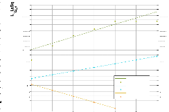
100000

100000

				Order x C5ALSq Order x C5A Order x C5LLSq Order x C5L Order x C5NLSq Order x C5N

10000000

10000000

50000

50000

5000000

5000000

2000000

2000000

20000

20000

1000000

1000000

10000

10000

500000

500000

5000

5000

200000

200000

100000

100000

2000

2000

50000

50000

1000

1000

20000

20000

10000

10000

500

500

5000

5000

200

200

2000

2000

1000

1000

100

100

500

500

50

50

200

200

Order x C5ALSq Order x C5A Order x C5LLSq Order x C5LLSq Order x C5NLSq Order x C5NLSq

20

20

100

100

50

50

10

10

20

20

5

5

10

10

5

5

2

2

2

1

1

1

1

1 2 3 4 5 6 7

Order

1 2 3 4 5 6 7

Order

Figure 25 Horton morphometric parameters for 4 selected sub-watersheds in the Congo River

37

Table 9 Horton Morphometric Parameters for the sub-catchments in the Congo River.

Sub- watersheds	RB	RL	RA
Ouesso	3.2	2.4	3.5
Sangha South	5.1	1.7	6.1
Ubangi	4.0	2.2	4.3
Kasai	2.7	1.6	3.3
Lualaba	4.2	2.3	4.6
MIN	2.7	1.6	3.1
MAX	5.1	2.5	6.1

4.4.2.2.2 Law of Stream Lengths and stream length ratio (RL)

The stream length assumes that the average lengths of the streams of successive orders are related by a length ratio RL, and given by the equation:

(22)

L

R thus L L R

= = ×

i

^L L +

1

i i L

1

i +

Table 10 Stream Length Ration for the different sub-catchments in the Congo River

		Ouesso	Sangha	Ubangi	Kasai	Lualaba
		C1_L	C2_L	C3_L	C4_L	C5_L
Stream Order	1	64.74	64.76	65.19	77.44	57.51
	2	196.02	183.8	191.43	234.59	185.49
	3	384.32	189.49	340.46	476.94	346.48
	4	662.01	664.74	932.09	82 1.84	98 1.2
	5	0		2130.4	1013.09	2265.76
	6	0	0	0	1152.81	0
	7	0	0	0	0	0
Horton Ratio	RL	2.44	1.71	2.21	1.64	2.3

The stream length ratio values (Table 10) fall between the natural limits ranges of 1.6 - 2.5 (MacCuen, 2005).

1 2 3 4 5 6 7

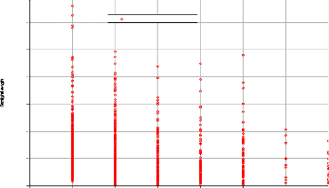
Strahler x StraightLength

300000

250000

200000

150000

100000

50000

0

Strahler

Figure 26 Strahler order vs. Stream length map

Above (Figure 26) is a plot of Strahler stream order and stream length. It is evident form the figure that this region has well defined geomorphic features with stream length of 1 st order streams varying from 3 km to 335 km, and 7th order streams with length varying from 0 to 90 km. Also, the stream number in a subwatershed is inversely correlated to the stream order (FigurF26).

4.4.2.2.3 Stream Area Ratio (RA)

Stream ratio is given by the following equation and the obtained values from the DEMHydro processing are presented in Table 11 bellow.

R_A

A i + 1

= (23)

A_i

Table 11 Stream Ration for the selected subwatershed

		Ouesso	Sangha	Ubangi	Kasai	Lualaba
		C1_A	C2_A	C3_A	C4_A	C5_A
Stream Order	1	3322.57	C2_A	3137.12	2986.6	2591.04
	2	21035.86	3258.19	15777.09	16796.23	16541.88
	3	49761.68	14855.7	61493.83	63232.86	70292.39
	4	158672.2	119366.6	296725.4	177175	358082.7
	5	0	132257.5	646792.4	450879.8	1121600
	6	0	0	0	905331.4	0
	7	0	0	0	0	2445.2
Horton Ratio	RA	3.5	6.05	4.34	3.25	4.6

4.4.2.2.4 Channel slopes and length

The steep slope of a watercourse favours and accelerates the runoff, while a small slope gives the water the necessary time to infiltrate totally or partially into the soil. The calculation of the average slope is obtained from the longitudinal profile of the main stream and its tributaries.

The most frequent method used to calculate the longitudinal slope of a watercourse consists of correlating the difference of altitude of the extreme points of the stream with its length.

Si

ÄH (24) L

where: S1 longitudinal slope of stream [m/km] or [%o]

?H: difference of altitude of the extreme points of the stream [m]
L: total length of the stream between its extreme points [km]

At a spatial resolution of 1 km (Hydrosheds and Hydro1k) the slope values for each pixel grid seems to be negligible.

4.4.2.2.5 Channel degree of development

Drainage density, introduced by Horton, is the ratio of the total length of streams within a watershed to the total watershed area (Equation 24).

Dd L i = ?

(25) A

where: Dd: degree of development of the hydrographic network [km/km2], Li: length of the stream [m] and A: watershed surface [km].

The Density values for each subwatershed are given in Table 12. The subwatershed density varies between 22.6 and 27.6 with a mean of 24.2 and a standard error of 0.63. A high value of stream density indicates a relatively high density of streams and thus a rapid storm response. The development of stream seems to be uniform all over the basin.

Table 12 Drainage density for watersheds of the Congo River

ID	1	2	3	4	5	6
Name	Ouesso	Sangha South	Ubangi	Kasai	Lualaba	Congo	CRB
A (Km2)	155408	130671	639564	895179	1109014	849063	3778879
Li (m)	3572.4	3117	15455.1	25007	27362.9	19436.5	93953.5
Dd (m/Km2)	22.73	23.59	23.9	27.62	24.4	22.64	24.6

Owing to the fact that all the Horton geomophometric parameters fall in the accepted natural limits, we assume that the 5 sub-watershed extracted from the DEM are representative for the Congo watershed and can therefore be used in the GIS-linked hydrological model to develop.

4.5 GIS-Based Hydrological Model Development

4.5.1 Introduction

In order to compute the water resource availability and to simulate the spatial and temporal distribution of water balances over the Congo River Basin (CRB), a GIS-based hydrological model, namely HATWAB (Hybrid Atmospheric and Terrestrial Water Balance) was developed and parameterized for the Congo basin (Figures 27 and 28), based on the initial model of Alemaw (2006). Initially, a GIS based hydrological model (Alemaw, 1999) was developed to computer the spatial and temporal distribution of water balance in southern Africa reion. This model was modified and used for the same region (Alemaw and Chaoka, 2003) and for the Limpopo basin (Alemaw, 2006). The approach of this model is based on the parametersization of input data, viz monthly temperature, precipitation, land-cover/use, soil texture and rooting depth and the Digital Elevation Model, to compute temporal and spatial variability of water budgets at geo-referenced grids cells covering the Congo basin.

The atmospheric component of the water balance model computes the Integrated Vertical Moisture Convergence (C) based on the precipitation and evaporation, while its terrestrial component estimates Actual Soil Moisture (SM), Actual Evapotranspiration (AET), and Runoff (TRO). Surface abstractions components in term of overland runoff (DRO) and interception are also accounted. The model estimates the uncertainties on water balance parameters and as well as the imbalances.

A separate component of the model consists of a DEM hydrological processing. This component extracts watershed and streams network (Figure 12), compute their hydrogeomorphometric parametes which characterise the topography, topology and hydrography of the river basin.

The Spatial and temporal distributed water balance model requires various types of data from different sources (Melesse et al, 2006) like Remotely-sensed datasets (NDVI images, DEM), meteorological datasets (precipitation, air temperature, wind speed, sunshine hours, etc), hydrologic (river discharge), hydrologic soil maps and other GIS layers ( watershed boundaries and properties, streams topology, etc) in raster,vector and tabular formats. Their collection and preparation will be presented in section 5.4.

Figure 27 General terrestrial Water Balance model structure

RAINFALL
(PPT)

Surface process

EPPT = PTT -DRO

EFFECTIVE
RAINFALL
(EPPT)

DIRECT RUNOFF (DRO)

Soil storage

(FC, WP, AWC...)

Excess =
EPPT- DRO - AET-? SM

RUNOFF
STORAGE
(RO)

TOTAL
RU NO FF
(GRID)

ACTUAL
EAVPO-
TRANSPIRATION

Figure 28 Rainfall-Runoff simulation model for a single grid cell

4.5.2 Water Balance Model development procedure

The water balance model development comprises the following steps:

(i) Vertical Integrated Moisture convergence:

The Vertical Integrated moisture convergence (C) is a component of the atmospheric water balance and will be computed based on rainfall and Evapotranspiration data.

(ii) Rainfall-Runoff Development

At this stage, components derived from previous steps will be used to generate monthly water balance compounds as shown in Figures 27 and 28: Runoff (TRO), Actual Evapotranspiration (AET), Soil Moisture (SM) and Percolation (P). The Thornthwaite and Mather (1957) method, slightly modified, generate a monthly water balance for each grid-pixel as well as for the whole Congo River Watershed.

(iii)DEM-Hydro processing: Watershed and Streams delineation

Watershed and sub-watershed boundary maps are required to delineate the specific area where the soil-water balance model will be applied. In other words, the model will account for the water balance for the grid cells falling in the watershed limits. These files, namely `MASKS', are extracted during the DEM processing.

The DEM-Hydro Processing were developed in section 4 in order to derive Geomorphometric properties of the catchments and stream network like flow direction, flow accumulation, catchment, drainage network, overland flow, masking files, and other hydrologic data using GIS packages (viz ILWIS 4.3 and ESRI ArcMap 9.2 versions). The Horton statistic parameters were used for discriminating and characterizing the extracted watershed and streams from the DEM.

4.5.3 Water Balance Model Development

Supposing the principle of continuity in hydrologic system, Chow (1998) assumes that the time rate change of storage is equal to the difference between the input and the output in of the hydrologic model (equation 26).

ds I O t= - t t dt

(26)

where, St is the time-variant storage in a grid cell, It , the summation of input coming into the cell from upstream cells and the runoff generated in the cell, and Ot , the outflow from the cell which is calculated by various methods, e.g. the linear reservoir method.

4.5.3.1 Atmospheric water balance

The atmospheric component of the water balance model is expressed as

^dWPEC

dt = - + + (27)

C=-?×Q (28)

Where dW/dt is the amospheric storage change, C is the vertical integrated moisture converence (LT^-1) and was expressed as a function of the water vapour flux (Q) in Equation (28).

? × Q is the divergence or net outflow of water vapor across the sides of the atmospheric column, Q is the vapor flux, E is evaporation, and P is precipitation.

The quantity W is also referred to as the precipitable water and may be expressed in units of mass per unit surface area [M L^-2] or converted to an equivalent depth of liquid water [L] by dividing by the density of liquid water (1000 kg m^-3).

The divergence Q mesures the difference between inflow and outflow to a region; a positive divergence means that outflow is greater than inflow, and a negative divergence (or convergence) means that inflow is greater than outflow. The units of divergence are [M L^-2 T^-1] but may also be expressed as depth of water per time [L T^-1].

In mean water balance computation like the HATWAB model which is monthly water balance model, the atmospheric storage change is often assumed to be negligible (Reed et al, 1998 and Marengo, 2005); thus equation (28) is reduced to

P-E=C or P-E=-?Q (29)

From Equation (30), it is seen that if the divergence (?Q	) in a region is positive, then

evaporation is greater than precipitation (P-E < 0), while a negative divergence or "convergence" indicates that precipitation is greater than evaporation (P-E > 0).

4.5.3.2 Terrestrial water balance

At monthly time scale a terrestrial water balance model is written as

ds P E R

dt = - - (30)

Where S is soil moisture storage (L); P is precipitation (LT^-1); E, actual Evapotranspiration ((LT^-1); and R, the observed runoff (LT^-1).

Linearising Equation (30), the terrestrial water balance has the following form

SM₁ = SM t - 1 + P _t -E t - R t (31)

Where t is the time period, which is a single month is this model, P is precipitation, E is the Evapotranspiration, and RO is the runoff.

Once the initial soil moisture _(St-1) and the actual soil moisture (St) are determined, the monthly Actual Evapotranspiration Et and the Runoff Rt can be calculated.

4.5.3.3 Imbalance estimation

Combining Equations (30) and (31), the vertical integrated moisture convergence (C) is computed as follows

dS
C R

- = (32)

dt

In a steady state P AET =R. Changes in storage could however lead to P E being different from R. These could also be due to certain errors in representing rainfall within the Congo River Basin. These lead to the expression of an imbalance equation

C ds dt R

- ( / + )

Imb = (33)

R

The imbalance in _Imb is calculated using the following formula:

C ds dt

/

Imb (34)

= - + 1

R R

Contrary to the formulation adopted in this study based on (34), Marengo (2005) assumes that dS/dt is negligible for monthly time scales and applied it in the Amazon basin, which reported unaccounted residuals in his water budgets. Whereas in the proposed model in this study, the soil moisture variation dS/dt is varying from season to season as a function of the prevailing PET and PPT at a given location according to Equation (30), in which the imbalance should also cater for this variability according to Equation (34). One of the contributions of this study is that, once the imbalance (Equation 34) is kept to a minimum in the water balance computation at each grid, then the simulated variables and water balances, PPT, ET, RO, RO/PPT, ET-PPT, ET/PET, S and C can then be used to investigate the seasonal and temporal variability of water budget of the Congo basin.

The amount of precipitation and potential evapotranspiration determines soil moisture availability, which in turn is controlled by the water holding capacity of the soils. Solution of the mass balance equation will be solved for E, R and S (section 4.5.3.4).

4.5.3.4 Rainfall-Actual Evapotranspiration-Soil moisture-Runoff modelling 4.5.3.4.1 Effective Precipitation (EPPT) and overland runoff (Direct runoff DRO)

One of the main inputs required in the proposed water balance model is the effective precipitation (EPPT). At a monthly time scale, the effective precipitation is calculated as per the formula of the USDA soil conservation available from FAO (1990) as follows:

125 0.2

- PPR

EPPT PPT for PPT mm

= ( ) 250

< (35)

125

EPPT = 125 + 0.1 PPT forPPT=250 mm (36)

Where EPPT is effective precipitation and PPT is the total precipitation

The direct runoff (DRO) is the difference between the precipitation (PPT) and the Effective precipitation (EPPT).

4.5.3.4.2 Soil moisture estimation (SM)

Soil moisture is determined from the interaction between effective PPT and PET. During wet months (when effective PPT in excess of PET), soil moisture can increase up to a maximum of field capacity determined by soil texture and rooting depth.

dt

dSM = EPPT - PET when EPPT > PET and SM < FC (37)

dt

dSM = 0 when SM = FC (38)

dSM ( - )

dt

= a SM PET EPPT when EPPT < PET (39)

Where, FC is the soil moisture at field capacity of the soil millimetres, PPT is precipitation in mm/month; PET is potential evapo-transpiration in mm/month.

During the dry periods where the EPPT < PET, the soil becomes increasingly dry, soil moisture becomes a function of potential soil loss. Thus, different authors assumed different relationship to find the soil moisture during the dry periods (Thornthwaite, 1948; Vorosmarty et al., 1989).

For a particular soil, there is a linear relationship between Log (SM) and Ó(EPPT-PPT) summed from the start of the dry season to the current month. Thus, to calculate the rate of change of soil moisture (ÄS) through the dry season, the soil moisture is directly estimated from the empirical relation suggested by Vorosmarty et al. (1989). To calculate ÄSM/dt through Equation (40) for intermediate field capacities, the HATWAB defines a slope a to the retention function as:

a = ln(FC)/(1.1282 FC)1 . 2756 (40)

where the numerator represents soil moisture (millimetres) with no net drying. The
denominator is the accumulated potential water loss or APWL ( ? [PET - PPT ]) in mm

at SM=1 mm. With a determined, the model can calculate dSM/dt as a function of soil dryness and update SM. Figure 29 shows the relationship between soil moisture and the Evapotranspiration. Between the plant wilting point and the root zone Field Capacity, Evapotranspiration increases with the soil moisture.

Calculations commence at the end of the wet season when it is assumed the soil is at the field capacity. Soil water stocks are then depleted during the dry season in accordance with the moisture retention function. For each wet month, soil moisture is determined by incrementing antecedent values by the excess of the available water over PET. This recharge may or may not be sufficient to bring the soil to field capacity at the end of subsequent wet season.

ETa/ETp

1

WP FC=WH

SM

Figure 29 Functional relationship between soil moisture and Evapotranspiration (ETa is the actual Evapotranspiration, ETp is the potential Evapotranspiration, SM is the soil moisture, FC is the field capacity and WP, the Wilting point

Analysis of the ratio PPT/PET at the various grids in Central Africa has shown that the region can not be represented by one homogeneous climatic zone, rather it is a combination of climate influenced by the diversified hydro-climatic conditions in the region. In this analysis, it has been observed that the long-term monthly rainfall distribution varies greatly in the region.

It is assumed that the ratio PPT/PET could be a good indicator of the seasonal distribution of monthly rainfall, and accordingly the wet season ends when the ratio PPT/PET just starts to fall below unity. In line with this, therefore, the soil moisture can be assumed to be at its field capacity. Consequently, HATWAB fixes a starting month of any grid across the region according to the aforementioned criterion. The solution of the basic mass balance equation for the subsequent months can determined once the initial soil moisture state is obtained.

4.5.3.4.3 Actual Evapotranspiration (AET)

Once the actual soil moisture is determined, the corresponding actual evapotranspiration (AET) is calculated for the month. Following the Thornthwaite and Mather (1957) approach, AET is set equal to PET in wet months, when EPPT > PET. During this time it is assumed that EPPT is in sufficient abundance to satisfy all the potential water demands of the resident vegetation. During dry season when EPPT < PET, the monthly average AET is modified down wards from its potential value as shown below.

AET = PET when EPPT > PET (41)

dSM

AET = EPPT - when EPPT < PET (42)

dt

where the soil moisture drops below the wilting point, the AET is equal to the EPPT but if there is no EPPT at all time, AET becomes zero.

4.5.3.4.4 Total runoff (TRO) generated at a grid spatial scale

Most of the water does not leave the basin as soon as it becomes available as surplus. The
portion that constitutes overland flow is assumed to flow out of the watershed within the

month it occurs but the portion that infiltrates may take a number of months to move slowly through upper layer of the soil column to emerge in the surface water courses as base flow.

The lag or delay factor depends not only the size of the basin but also on the vegetation cover and the soil type, degree of slope, characteristics of the soil layers, etc. Thornthwaite suggested that 50 % of the water surplus could be assumed to runoff each

month from large basins with the remainder being held over and added to the surplus of the next month. This factor is set according to Thornthwaite & Mather (1957) which is equal to 0.5.

RO = (D + (EPPT - PET) when SM = FC EPPT > PET

0 . 5 * ) &(43)

RO = 0.5 * D when SM < FC EPPT < PET

& (44)

Where, RO is rainfall-driven runoff or surplus runoff (mm/month) and D is the amount of detention storage in millimeters that is assumed to leave each grid cell next month.

4.5.4 Data sets and software

This study requires a set of hydro- meteorological variables (rainfall, evapotranspiration, and wind speed), topographic data or Digital Elevation Model (DEM) data set, landcover/use variables, vegetation, soil data.

4.5.4.1 GIS and geo-referencing procedure

The Congo River basin has a sub-continental extension covering 8 countries in Central Africa region. It is extended between 15⁰S to 10⁰N and 10⁰E - 35 ⁰E. Originally, the area of study has a spatial resolution of 30x30 minutes but for a better resolution and accuracy of the results a 6 minutes (averaged to 12km at the equator) was adopted and forced by the computational techniques.

The Kriging method (Krige, 1966; Stein, 1998, Surfer v.8) was used to interpolate and fill the missing value, harmonizing different data sets to a spatial resolution of 6 minutes for a single grid cell, corresponding to 62500 square grids (250 rows and 250 columns).

4.5.4.2 Meteorological data sets

Free meteorological data for 3262 global climatic stations are available at FAO-UNESCO /CLIMWAT, with a record time of 30 years (1961 -1990) at a monthly scale; where 145 climatologic stations covering the study area (Figure 29 and Appandix 1) were extracted to compile the meteorologic database for the model. These climatologic data sets include monthly averages of maximum and minimum of temperatures, mean relative humidity, wind speed, sunshine hours, radiation data as well as rainfall and Reference Crop Evapotranspiration (ETo) calculated with the Penman-Monteith method (Allen et al, 1998). Below, Figures 31 and 32 show the Rainfall and Potenital Evapotranspiration distribution in the basin, respectively.

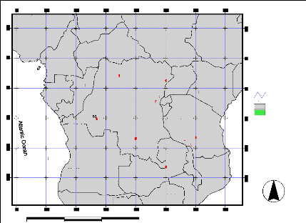
700 0 700 1400 Kilometers

Enugu

%

Kano

Libreville

Pointe Noire

%

Douala

%

%

Malabo

%

Port Gentil

%

Benguela

$

Luanda

Yaounde

%

Brazzaville
$

$

$

%

$

$$

M $

atadi $ $

%

$

$

%

$

$

$

$

% %

Huambo

%

Maiduguri

$ $

$

$

$

$

$ % %

%

$

$

$

$

Kinsha

$

$

$

$

$

$

Mbandaka
$

$

$

$

$

$

$

Kahemba

%

Bangui

$ %

$

$

$

%

$

$

$

$

$

$
$

$

$

$

$

$

$

$

$

$

%

$

$

$

$

$

Kananga $ $ $

$$

$ $

$

$

$
$

$ Kisangani

$ $ %

Lumumbashi

$ $

Livingstone

$ $

%

$

$

$

$

$

$

$

$

$

$

$ Kigoma

$

%

$

$

$

$

Lusaka

$$ %

$

$

$

$

$ $

%

$

$

$

$ $ $

$

$ Kigali

%

$

$

$

$

^%Bujumbura

Harare

$

$

$

%

Kampala

%

$

$ $

$

$

$

$

$ Lilongwe

%

$

$

Dodoma

$

$

$

$

Beira

$

Dar es Salaam

Nairobi

%

Adis Abeba

Mocambique

%

%

Mtwara

%

%

%

Mombas

%

Djib

An

$ Stations zxy.txt

% Cities.shp

Afrbord.shp

Afpolit.shp

Latlong.shp

Figure 30: Distribution of Climatic stations in the study area. The study area covers more than 145 stations

10

-10

-15

-5

5

0

Annual Rainfall							mm/year 2100 1900 1700 1500 1300 1100 900 700
Annual Effective	Rainfall					mm/year 1600 1500 1400 1300 1200 1100 1000 900 800 700 600

10 5 0 -5 -10 -15

10 15 20 25 30 35 10 15 20 25 30 35

10 15 20 25 30 35

10 15 20 25 30 35

Figure 31 Rainfall averaged (1961-190) data from 145 stations. 1. Rainfall, 2. Effective Rainfall

10 5 0 -5 -10 -15

Annual Potential

	Evapotranspiration			mm/year 1800 1500 1400 1300 1200 1100 1000

10 15 20 25 30 35

Figure 32 Mean Annual Potential Evapotranspiration (1961-1990) map

4.5.4.3 Discharge data

There is a lack of discharge data in the Congo Basin although there is Rainfall gages and data since 1958. The availability of recharge data is limited to a few numbers of rivers gauges. At the basin final outlet, discharge has been amounted to an average of 45000 m³/sec (Asante, 2000).

Discharge data indicate a series of four distinct phases in the Congo and the Oubangui since the beginning of the 20^th century. During the 1 960s they increased, overtaking their average over a century. The Congo discharge then fell, returning in 1970 to what had been the normal level, whereas the Oubangui entered a drought phase. This trend accentuated from 1980 and, until 1996, the Congo discharge weakened by 10% (37 400 m3/s in 1992 compared with an average of 40 600 m3 /s over that period as a whole), which was the most dramatic decrease of the century. This fall is much stronger in the Oubangui (- 29%), yet negligible (- 0.2 %) in the Kouyou sub-basin. Overall, whereas discharge decrease in the Congo Basin is between two and four times the drop in rainfall (IRD, 2002) Table 14 summarises the Congo River discharge (1903 -1983) at Kinshasa station.

4.5.4.4 Digital Elevation Model (DEM) and Mask files

The topographic properties of the area were derived from a DEM raster data namely HYDRO1k. The HYDRO1k is a geographic database developed at the U.S. Geological Survey's EROS Data Centre to provide comprehensive and consistent global coverage of topographically derived data sets, including streams, drainage basins and ancillary layers derived from the USGS' 30 arc-second digital elevation model of the world (GTOPO30).

The HYDRO1k has the advantage of being hydrologically corrected for calculation of derived hydrologic parameters such flow direction, flow accumulation, slope (Asmamaw, 2003); and it is freely available at a standard suite of geo-referenced data sets with a spatial resolution of 1 kilometre, adapted for a large scale water balance model. Figures

14 and 21 show the DEM of the study area and the polygon map of the entire CRB and sub-watersheds `Mask files».

4.5.4.5 NDVI and vegetation database

The monthly NDVI images for each basin were acquired from the Global Land Cover Characteristics database. Satellite data have been used extensively for mapping the land use and for monitoring the seasonal change of vegetation of river basins (Nemani & Running, 1989).

The Normalized Difference Vegetation Index (NDVI) is commonly applied to derive the leaf area index (LAI) from channels 1 and 2 of NOAA-AVHRR data at 1 -km² resolutions. Monthly twelve NDVI images, expressed in percentage, for 1987 are acquired from USGS web pages. Based on NDVI values the LAI for different land use groups can be estimated by empirical formulae. Table 13 presents rooting depth assigned for various soil textures and SCS soil groupings

Table 13 Rooting depth assigned for various soil textures and SCS soil groupings

Veg. Group	NDVI	Assigned Root Depth (M) For Different Soil Types
		Sand	Sandy Loam	Silty Loam	Clay Loam	Clay	Lithosol
VEG2	>50%	2.5	2.0	2.0	1.6	1.2	0.1
VEG1	=50%	1.0	1.0	1.3	1.0	0.7	0.1
SCS soil group (Singh, 1992)		A	B	D	C	C	B

4.5.4.6 Soil properties

A global Soil map at 10x10 minutes resolution is freely available at FAO/UNESO database (FAO, 1984). This map is used to extract the submap of the study area and later re-sampled to a spatial resolution of 6x6 minutes so that it can overlay onto the model.

Since the Soil Water available to plants depends on soil water content, soil texture (Figure 33), and consequently, the rooting depth of vegetations, the 133 agronomic groups of FAO agronomical soil map were therefore used to derive and reclassify textural soil classes which are required as input data for the model. For this matter a FORTRAN algorithm was developed and 6 hydrological textural classes of soil (Table 14 and 15) were identified in the study area.

Table 14 Soil texture distribution in the Congo River basin

Class ID	1	2	3	4	5	6	0	Total
Soil type	Sand	Sandy Loam	Silty Loam	Clay loam	Clay	Lithosol	Water body
No grids	4847	0	58	21867	989	2374	513	30640
% gris	15.8	0	0.2	71.3	3.2	7.7	1.7	100

The reclassified textural soil and vegetation maps are used to derive the soil retention parameters such as Field Capacity (FC), Wilting Point (WP) which determine the soil moisture capacity known as Available Water Content (AWC) for each soil group.

Based on field measurements, Saxton et al. (1986) have developed a technique to estimate the matrix potential of different soils by using multiple regression techniques. Therefore, at a matrix potential equivalent to field capacity (33 KPa) and wilting point (1500 KPa) for a unit meter depth of soil, approximate values of FC and WP for the various soil textures have been extracted (see Table 15). Accordingly, the FC and WP values as per the rooting depth are then derived for the whole region as summarised in Table (15). Available water content (AWC) of a soil of given texture is defined as the difference between the field capacity and wilting point.

The depth of soil water which can be used by the crop, the Total Available Water (AWC), depending on the root depth of the crop and on the soil moisture holding properties of the soil (Eilers et al, 2007), Equations (45, 46) bellow shows the relationship between these soil parameters:

AWC = (UFC-UWP)R (45)

With

FC UFC R = × WP UWP R = ×

(46)

Where AWC is the available water content per root depth; FC and WP are the field capacity and wilting point, respectively; R is the current depth of the roots; UFC and UWP are the field capacity and the wilting point per unit volume of the soil, respectively.

Figures 33-36 show the generalised relationship between the soils parameters, the Textural soil groups, the Field capacity map, the Wilting Point map and the Available water content map, respectively.

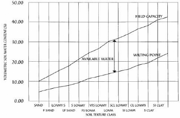
Figure 33 Available soil water vs. soil texture showing estimates of field capacity, permanent wilting point and Available water content. S-Sand, SI-Silt, CL-Clay, F-Fine, VF-Very Fine, L-Loamy (after Levy et al, online)

Table 15 Relationship linking vegetation class, soil texture, rooting depth and moisture capacities of various soil groups in Central Africa (Source: Alemaw and Chaoka, 2003)

	Sand Sandy Loam Silt Loam Clay Loam Clay Lithosol
Veg. Group	The Root depth (m)
GRP1	2.5	2.0	2.0	1.6	1.2	0.1
GRP2	1.0	1.0	1.3	1.0	0.7	0.1
2.3.2.1.1.1.1.1.1 FC and AWC of soils as % of total volume of soils / m
% (FC)/m %(AWC)/m	14.1 6.3	20.0 9.1	27.3 13.2	35.2 35.8	48.5 35.8	27.3 13.2
2.3.2.1.1.1.2 Field Capacity and AWC per root depth of the plant
GRP1 (FC) (AWC)	353 196	400 218	546 282	563 243	582 153	27 14
GRP2 (FC) (AWC)	141 78	200 109	355 183	352 152	339 89	27 14

-10

-15

10 15 20 25 30 35

10

-5

5

0

Textural Soil Types map						Soul types 6 Luthosol 5 Clay 4
						Clay loam 3 SultLoam ^2Sandy Loam 1 Sand
						0 Water body

Figure 34 Hydrological Soil types over the basin

10 5 0 -5 -10 -15

Soil Fiel Capacity in the root zone					mm/root depth
						0	550 500 450 400 350 300 250 200 150 100 50

10 15 20 25 30 35

Figure 35 Soil Field Capacity in the root zone.

10 5 0 -5 -10 -15

Soil Available Water Content					mm/root depth
						0	240 220 200 180 160 140 120 100 80 60 40 20

10 15 20 25 30 35

Figure 36 Hydrological Soil types over the basin

4.5.4.7 Software resources

The packages used in this research are FORTRAN Power Station, ILWIS 3.4, ArcGIS 9.2, ArcViewGIS 3.3, Canvas7, Surfer v8.0 and CorelDraw v12, and Microsoft Excel packages.

CHAPTER FIVE

5.0 MODEL APPLICATION, DATA PRESENATTION AND INTERPRETATION RESULTS

5.1 Generalities on the Model application

The HATWAB model runs and simulates the water balance for each of the 62500 grid cells of the study area using inputs datasets previously developed and presented in GIS dataset formats. The GIS-database includes the hydro-climatic data sets which are potential precipitation (PPT) and potential Evapotranspiration (PET). It includes also the soil texture, the Vegetations, and rooting depth, which are used to derive the Soil moisture capacities per unit volume: Field capacities (FC), Wilting point (WP), Available water content (AWC). All the data sets are incorporated in the model at a 6X6 minutes (12X12 km) grid cell spatial resolution.

A raster file having an integer value of 1 inside the basin area and 0 outside the basin is assigned to the model as masking file delineating and forcing the basin boundary to the entire output of the model simulations.

Other important characteristic of the model is the facility to simulate the water balance for a specified area: a single grid cell, a sub-watershed (example: Kasai, Ubangi, Bangui, Ouesso, Lualaba sub Congo) or the entire Congo basin.

For each grid cell, the model run for a time loop of 12 months, using PPT and PET data sets available for a period of the 30 years (1961-1990) until a dynamic steady state is achieved in SM, AET and TRO with tolerance error of 0.01% in all these variables. If the steady state is not achieved the model proceed on a second, third, and so on, until the steady is achieved.

Finally, monthly and annual averages for Soil moisture (SM), Actual Evapotranspiration (AET), Runoff (TRO), Vertical Integrated moisture coverage (C), and the Imbalance (I) are outputted for the entire basin.

A spreadsheet was developed to accumulate the total Runoff for each sub-watershed, and to average the annual Soil moisture and Evapotranspiration. These results will be presented in the following sections.

5.2 Initial soil moisture

In order to solve the water balance differential equation governing the soil moisture Equation (31), the initial soil moisture is determined in accordance with Alemaw (2003). In most hydrological water balance, it is assumed that at the end of a wet season the soil moisture remains at the state of its field capacity attained during the wet season. Therefore, the simulation starts at the end of the wet season when it is assumes that the soil is at field capacity. Soil water stocks are then depleted during the dry season in accordance with the moisture retention function.

For a large watershed, the ratio PPT/PET can be used as a good indicator of seasonal
distribution of the wetness of the dryness at a specific geographic location in a region: a
wet season is characterised by a ratio PPT/PET greater than the unity, while a value less

than the unity corresponds to the dry season. The month where PPT/PET just starts to fall under the unity is selected by the model as the starting month of the simulation.

5.3 Data presentation and Interpretation results

5.3.1 Soil moisture (SM)

Annual average Soil moisture and seasonal soil moisture maps are shown in Figures 38 and 39, respectively. The mean annual soil moisture for the entire basin ranges between 0.7 and 431.4 mm, with highest mean monthly soil moisture of 546.2 mm during November and lowest, in July (146.2mm). A general trend is observed in the spatial distribution of the moisture: the regions around the equator are characterised by high soil moisture and this is reduced as the distance to equator is increased (Figure 37).

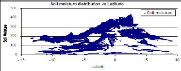
Figure 37 Soil moisture correlation with the latitude

Spatially, the highest values are located in the centre of the basin which coincides with the core of the dense equatorial forest. These values range between 200 and 432 mm (mean annual). The lowest value ranging between 0 and 50 mm are located in the western part on Tanzania (eastern part of Tanganyika Lake). This region is also characterised by the small amount of annual rainfall (< 800) compared to other region inside the basin, «Lithosol» as type of soil Available Water content (<120 mm/root depth).

Statistically, the soil moisture distribution over the basin correlates strongly with the hydrological soil group and the climatic parameters such as rainfall and Evapotranspiration. The computed soil moisture values would be better interpreted as indexes of relative wetness rather than absolute estimates because none are calibrated against measured values in the field.

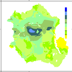
Soil Moisture

mean ann (mm)

250

200

350

300

50

0

150

100

10

5

0

-5

-10

-15

10 15 20 25 30 35

Figure 38 Mean annual moisture (in mm) over the Congo basin.

10 15 20 25 30 35

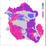
Total Soil Moisture- June-July-August (mm)

400

300

200

100

0

10 15 20 25 30 35

10 15 20 25 30 35

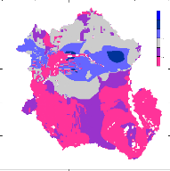
Total Soil Moisture- September-October-November (mm)

500

400

300

200

100

0

10 15 20 25 30 35

10

5

0

-5

-10

-15

10

5 0

-5

-10 -15

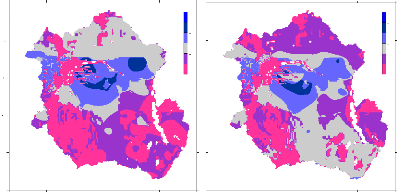
-10

-15

10

-5

5

0

-10

-15

10

-5

5

0

Total Soil Moisture- March-April-May (mm)

500

400

300

200

0

100

Total Soil Moisture- December-January-February (mm)

500

400

300

200

0

100

Figure 39 Season Soil moisture (in mm per season) over the basin.

5.3.2 Actual Evapotranspiration (AET)

The simulated results for the Actual Evapotranspiration (AET) are monthly estimates for each 6 minutes grid cell covering the Congo basin. Figures 40 and 41 show the mean annual AET and seasonal AET, respectively. The mean annual AET ranges between 564.13 and 1576.8 mm/year with a mean of 1098 mm/year. It is well observed that the AET trends similarly with the Rainfall and the existing land cover map of the basin. Consequntly, the area with lowest AET is located in the south-eastern region of the basin which coincides with low rain feed region of the area.

-10

-15

10

-5

5

0

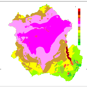
Total An nual Actual Evapotranspiration

mm/year

400

900

800

700

600

1600

1500

1400

1300

1200

1100

1000

10 15 20 25 30 35

Figure 40 Mean Annual Actual Evapotranspiration over the Congo River basin

High annual averaged AET values are sequentially observed over the water bodies such as the Tanganyika with a maximum of 1576.8 mm/year, followed by Upemba, Rukwa, Mweru, Delcommune, Bangwelungu Lakes (1300 - 1531 mm/year) and Kivu, Mai-Ndombe Lakes (>1250 mm/year). Some portions of the Congo River inside the heart of the Tropical forest present also high annual values of AET. Excluding the water bodies, the density of the equatorial forest varies positively with AET distribution.

The seasonal distributions of AET (FigurF41) are characterised by alternation of high values in the northern hemisphere during the two seasons of December-February and March-May and low values in the southern hemisphere; inversely during the other 2 seasons ( June-August and September-November).

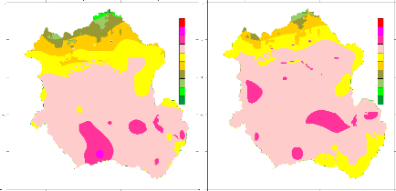
-10

10

15

5

0

5

-10

10

15

5

0

5

Actual Evapotranspiration: March-April-May

[mm]

400

250

200

500

350

300

150

100

50

0

Actual Evapotranspiration: December-January-February

[mm]

500

400

350

300

250

200

50

0

150

100

10 15 20 25 30 35 10 15 20 25 30 35

10

5

0

5

-10

15

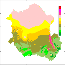
Actual Evapotranspiration: Jun-July-August

[mm]

500

400

350

300

250

200

50

0

150

100

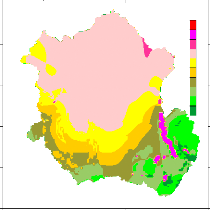
Actual Evapotranspiration: September-October-November

[mm]

400

250

200

500

350

300

150

100

50

0

10

5 0 5

-10

15

10 15 20 25 30 35 10 15 20 25 30 35

Figure 41 Season Actual Evapotranspiration over the Congo basin

5.3.3 Runoff

The simulated annual Total runoff is shown in Figure42. The mean annual Runoff for for the Congo Basin varies between 1 and 1945 mm with a mean annual runoff of 342 mm. The highest values are concentrated in the heart of the equatorial forest along the Middle Congo river branch. This area records higher rainfalls in the whole basin. The lowest value is simulated in the southern hemisphere around the grid of coordinate 31 ⁰E and and 6.73⁰S (western part of Tanzania). A part the lakes, the highest values of runoff are simulated in the heart of the equatorial forest across the equator, and decrease progressively towards the tropics. This trend is relatively disturbed with the soil types especially in the south-eastern, the extreme north regiond and along the main Congo River. The annual simulated runoff show a general trend strongly influenced by the distribution pattern of precipitation (Figure 43) in the basin, while seasonal and monthly runoff correlate strongly with both rainfall and soil type during dryer seasons. The area with zero runoff values correspond to swamps and some inland lakes where there is negligible or nil flow to the river system.

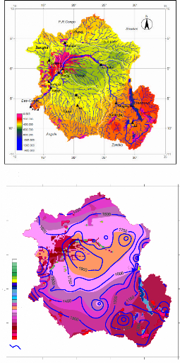
Figure 42 Mean annual runoff over Congo basin (mm/year)

10 15 20 25 30 35

10

5

Runoff

0

[mm/year]

1350

1250

1050

850

-5

750

650

525

400

350

-10

200

100

0

Rainfall

-15

Total Annual Rainfall and Runoff

Figure 43 The relationship between precipitation and drigged simulated runoff in the CRB

Seasonally, September-November records the highest amount (658432 mm. /season) of runoff whereas the lowest (358223 mm/season) is generated during June-August. This shows again the influence of rainfall on the generated runoff pattern in the Congo basin where, in general, the period June-July season records the lowest rainfall in the southern hemisphere which occupies more than 55% of the basin area. Two picks runoff are observed in March-May and September-November (658432 mm.) seasons which record higher rainfall during the year in the southern region.

Runoff: December-January-February

[mm]

450

400

350

300

250

200

50

0

150

100

10 15 20 25 30 35

10 15 20 25 30 35

Runoff: March-April-May

[mm]

450

400

350

300

250

200

50

0

150

100

10 15 20 25 30 35

Runoff: September-October-November

[mm]

450

400

350

300

250

200

50

0

150

100

10 15 20 25 30 35

10

5 0

-5

-10

-15

10

-10

-15

10

-10

-15

10

-5

-5

5

0

5

0

Runoff: Jun-July-August

[mm]

450

400

350

300

250

200

150

100

50

0

Figure 44 Seasonal Runoff grid runoff maps. Top left: December-February, Top right: March-May, Bottom Left: June-August, Bottom right: September-November

5.3.4 Simulated sub-watershed and basin-wide runoff

The runoff averages for each subwateshed are given in table 18 below. The Lualaba subcatchement knows the highest runoff than others. The higher amount accumulated runoff was expected in the Congo but this is not the case due to the presence of swamps in the subcachements where are simulated small values averaged to 0 mm per year.

At the basin scale, the total annual runoff is about 47,418 m³/sec. This amount is comparable to those reported in literature (45,000 m³/sec, Asante, 2000) with a marginal error of 5.1%.

Table 16 Subwatershed runoff averages

Area name	ROF ROF Simulated Mean Ann (m3/sec) (mm/year)	ROF Observed (m3/sec)	Error (%)
Sangha	335.5 3,565	No data	-
Ubangi	348.6 8,274	No data	-
Kasai	344.7 11,545	No data	-
Lualaba	297.3 12,3 14	No data	-
Congo	385.5 12,177	No data	-
CRB	342.0 47,418	45,000	+5.1

Figure 45 shows the local water balance graphs for 11 selected grid cells around selected rainfall stations used in the model. The hydrological behavior correlates strongly with the rainfall betwenn -5 and 5 degree latitude zone. In the South-eastern region (Lubumbashi, Urambo, South-westen) and the Up-North sation, runoff starts to increase in the mid-year as well as the soil moisture. An inverse situation is observed in the high rain fed region.

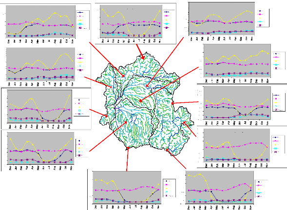
300

260

220

180

140

100

300
260 220 180 140 ^10060 20 -20	OUESSO
					AET PET PPT ROF SOM
300
260 220 180 140 100 60 20 -20		KINSHASA
			AET PET PPT ROF SOM
300
260 220 180 140 100 60 20 -20		KANANGA
				AET PET PPT
				ROF SOM
				300

-20

60

20

BANGUI

AET PET PPT ROF SOM

260

220

180

140

100

-20

60

20

Sangh

260

220

300

180

140

100

-20

20

60

SOUTH-WEST

Kasa

UP-NORTH

Ubangi

Cong

Lualab

AET PET PPT ROF SOM

AET PET PPT ROF SOM

300

260

220

180

140

100

60

20

20

300

260

220

180

140

100

-20

60

20

300

260

220

300

260

220

300

260

220

180

140

100

180

140

100

180

140

100

-20

60

20

60

20

20

60

20

20

LUBUMBASHI(-14, 27)

KISANGANI

BUKAVU (2852, -230)

BOYENDE

URAMBO

AET PET PPT ROF SOM

AET PET PPT ROF SOM

AET PET PPT ROF SOM

AET PET PPT ROF SOM

AET PET PPT ROF SOM

Figure 45 Local water balance for selected grid cells in the Congo River Basin.

5.3.5 Vertical Integrated Moisture Convergence

Figures 46 (A-D) show the Mean seasonal distribution of the Vertically Integrated Atmospheric Moisture Convergence (C) over the Congo Basin. The moisture convergence corresponds to the negative values whereas the positive values correspond to the moisture divergence.

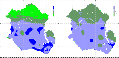
A

Vertical Convergence Moisture

CV'
Dec - Feb

2

0 0

-5

-5-5

-10

-15

10

-5

5

0

Vertical Convergence Moisture

B

CV'
Mar - May

-

-5-5

0 0

10

5

0

-5

-10

-15

10 15 20 25 30 35

10 15 20 25 30 35

10 15 20 25 30 35

10 15 20 25 30 35

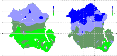
-10

-15

10

-5

5

0

Vertical Convergence Moisture

C

CV' Jun - Aug

2

0 0

-5

-5-5

-10

-15

10

-5

5

0

Vertical Convergence Moisture

D

CV'
Sep - Nov

-

-5-5

0 0

Figure 46 Seasonal and Spatial distribution maps for Vertical Integrated Moisture Convergence (in mm/month) over the Congo River basin. A: December-February, B: March-May, C: June-August, D: Septembre-November (Negative values correspond to the moisture convergence, positive values correspond to the moisture divergence).

The basin is well separated into two majors and disctintive zones based on the C parameter: The northern and the southern zones, corresponding exactelly to the northern and the southern hemisphere, respectively (Figures 46, A-D). Large values of Convergence (negative values) are simulated during June-August season (in the southern hemisphere) and December-February season (in the northern hemisphere), whereas during the same season, the northern and southern hemispheres are characterised by moisture divergence. During March-May season, the northern hemisphere sees its convergence moisture moving gradually towards the southern hemisphere, and a divergence moisture zone completely takes place at the end of June-August season. At the same time, the southern hemisphere which was characterised by the highest values of C during December-February starts to loose its C and

falls into a highest convergence moisture zone during June-August. This behaviour is clearly explained from monthly observations of C.

CHAPTER SIX

6.0 CONCLUSIONS AND RECOMMENDATIONS 6.1 Conclusions

The hydrogeomorphologic model has caracterised the Congo Basin in term of its topography, hydrography and hydrology. The major subwatershed (Sangha, Ubangi, Ouesso, Congo and Lualaba) are identical if considering the stream development characteristics. Slopes values are generally more or less negligible all over the basin. As observed from both the Hydrosheds and Hydro1k DEM maps used, more than 60 percent of the basin is covered by a flat area where slopes are obviously derived negligible. This flat area is surrounded by mountainous zones in the eastern, southern and northern part of the basin. The spatial resolution of 1000 meters used will definitely hide some ground realities such as hill slopes of a length less than 1000 metres, surrounded by flat area, will not be observed on the map.

Furthermore, a distributed GIS-based hydrological model, namely Hybrid Atmospheric Water Balance (HATWAB) was developed using GIS and computational hydrology techniques. The model is based on the combined, NDVI-based interception abstraction of precipitation, CN method of overland runoff and soil-moisture accounting technique for runoff generation for specific geo-referenced grids.

Besides, rainfall and climatological data, the inputs to the model are the GIS based agronomic soils and vegetation cover information over the region has been reclassified into appropriate textural soils and rooting depth and used to derive the soil moisture parameters such as field capacity (FC), wilting point (WP) and available water content (AWC).

This enables one first to establish the hydrologic regimes of the region, and for various drainage basins (subwatershed). It ultimately permits a through assessment of the region's water resources availability.

The simulated annual runoff using HATWAB for the Congo basin is found to be within 5% error margin compared to the observed mean annual runoff, which is quite a commending outcome of the study.

Developed for the water balance studies of drainage basins in the various climatic regimes of Africa, which is being successfully tested in different basins, HATWAB model is a regional scale hydrological model which is capable of estimating the spatial and temporal variation of the major components of water balance such as the soil moisture, the actual evapotranspiration and runoff.

First, the model has been used to create a GIS-based high resolution data sets of soil moisture, evapotranspiratiom, grid runoff for grids that represent the land catchment of the region at 12 km (6 minutes) spatial resolution.

This work is the first comprehensive distributed hydrological model in the region that utilises the hydro-climatology and hydrologic soil information using the state of the art GIS technique computing the water balance for the whole Congo River basin. The model and the findings of the study reveal important information to assess the water resources potential of the various sub-catchments and the whole Congo basin in one environment.

6.2 Recommendations

Even though the HATWAB model has simulated some realistic parameters for the Congo basin water balance, the following recommendations are made:

1. The soil texture data was not verified on the field. For the entire basin, only 6 textural soil groups were classified from 133 agronomical FAO soil groups. This may also introduced some error in estimation hydrological soil properties and therefore, in the simulation of water balance components.

2. The NDVI data was extracted from a map of 1987 while the climate change is affecting the Africa continent. There is a possible change in land cover/use distribution over the area.

3. Although the above mentioned deficiencies, one will need to point out that their influence would be negligible for such a HATWAB Model applied simulating the water balance for a large watershed such the Congo River basin. However, for further calibration of HATWAB model, observed or recoded discharge data for the various sub-catchment outlets as well as the main Congo basin outlet point need to be used.

4. With the advent of increasing computing power of the current computers, HATWAB can give an impetus to and can throw light towards development of refined and data intensive hydrological model as high resolution spatial and temporal hydroclimatic information are becoming increasingly affordable from satellite-data sources. Furthermore, this approach provides an operational hydrological tool to deal with national, or regional planning and developing decision support systems, with possible linkage with the inter-related multi-sectoral nature of the natural resources and socioeconomy of the region or the globe at large.

REFERENCES

Alemaw, B.F. and Chaoka, T.R. (2003). A continental scale water balance model: a GISapproach for the Southern Africa. Physics and Chemistry of the Earth, 28: 957-966.

Alemaw, B.F. (2006). A Hybrid Atmospheric and Terrestrial Water Balance Model. A GIS based approach for large drainage basins. Unpublished Research Report. University of Botswana.

AllAfrica, Central Africa: Congo River Basin Gets 2.44 Million Euros Grants From the African Water Facility. http://allafrica.com/stories/200706070044.html (accessed: June 2007)

Allen R. G., Pereira, L.S., Raes, D. and Smith, M. (1998). Crop evapotranspirationGuidelines for computing crop water requirements - FAO Irrigation and drainage. Paper 56. FAO, Rome

Arnell, N.W. (1995). Grid Mapping of River Discharge. Journal of Hydrology, 167: 39-56

Asmamaw A. (2003). Regional Scale Assessment and Modelling of Water Balance and Soil Erosion using global climate and Internet geodata sets: Case study of the upper Rio Grande System, Bolivia. M.Sc. thesis, ITC, Netherlands

Baumgartner, A., and Reichel, E. (1975). The World Water Balance. Elsevier, New York, 179 p.

Bergstrom, S., and Graham, L.P. (1998). On the scale problem in hydrological modelling, Journal of Hydrology, 211 (1-4): 253-265.

Beven, K. (1989). Changing ideas in hydrology-The case of physically-based models, Journal of Hydrology, 105: 157-172

Beven, K.J., Quinn, P.F., Romanowicz, R., Freer, J., Fisher, J., and Lamp, R. (1994). TOPMODEL. Computer Models of Watershed Hydrology. V.P. Singh (ed.), Water Resources Publications, Highlands Ranch, Colorado

BRICQUET, J.P. (1990) Régime et bilan hydrologique de l'Afrique Centrale. In : Paysages quaternaires de l'Afrique Centrale Atlantique. R. Lanfranchi et D. Schwartz (Eds). Publ. ORSTOM - Collection Didactiques. Paris p. 42-51.

Brubaker, K.L., Entekhabi, D. and Eagleson, P.S. (1994). Atmospheric Water Vapor Transport and Continental Hydrology over the Americas, Journal of Hydrology, 155: 407- 428

Butler and Rhett A. The Congo River- Rainforest Biodiversity. A Place Out of Time: Tropical Rainforests and the Perils They Face. (Accessed: January 2006 from http://rainforestsmongabay.com/0305.htm).

Chow V.T., Maidment, D.R. and Mays, L.W. (1988). Applied hydrology, MacGraw-Hill. pp.572.

Church, M. R., Bishop, G.D. and Cassell, D.L. (1995). Maps of Regional Evapotranspiration and Runoff/Precipitation Ratios in the Northeast United States, Journal of Hydrology, 168: 283-298.

Congo (2008). In Encyclopædia Britannica. (Accessed: March 2007, from Encyclopædia Britannica Online: http://www.britannica.com/EBchecked/topic/132363/Congo-Kinshasa)

Conway, D. (1997). A water balance model of the Upper Blue Nile in Ethiopia. Hydrologic Sciences Journal. 42(2): 265-286.

Costa, M. and Foley, J. (1999). Trends in the hydrologic cycle of the Amazon basin. Journal of Geophysical Research, 104:14189-14198

Curtis, S., Hastenrath, S. (1999). Trends of upper-air circulation and water vapor over equatorial South America and adjacent oceans. International Journal of Climatology, 19:863- 876.

Daly, C., Neilson, R.P. and Phillips, D.L. (1994). A Statistical Model for Mapping. Climatological Precipitation over Mountainous Terrain. Journal of Applied Meteorology, 33: 140-158.

Dunne, T. and Leopold, L. B. (1978). Water in Environmental Planning. W. H. Freeman and Company, New York, USA.

Eastman, J.R. (1997). IDRISI for windows user's guide. Clark University, Graduate School of Geography, Worcester, Massachusetts 06610, USA.

FAO (1984). FAO-UNESO soils map of the world revised legend, world soils resources report, series No. 60 Rome

Eilers, V.H.M., Carter, R.C. and Rushton, K.R. (2007). A single layer soil water balance model for estimating deep drainage (potential recharge): An Application to cropped land in semi-arid North-east Nigeria. Geoderma, 140:119-131.

Eltahir, E and Bras, R. (1994). Precipitation recycling in the Amazon basin. Quaternary Journal of Royal Meteorological Society. 120 (158):861-880.

Ewen, J., Sloan, W.T., Kilsby, C.G., and O'Connell, P.E. (1999). UP modeling system for large scale hydrology: deriving large scale physically-based parameters for the Arkansas-Red River basin. Hydrology and Earth Sciences System 3.1:125-136.

FAO (of United Nations) (1988) World Soil Resources, An explanatory Notes on the FAO world soil reference map, World Soils Resources Report, No. 66.

Gieske A. (2002). Viewer of ASC temperature and rainfall files per basin (CRU 1961-1990), ITC, Netherlands

Hay, L.E., and McCabe, G.J. (2002). Spatial variability in water-balance model performance in the conterminous United States. Journal of the American Water Resources Association, AWRA Paper 00086.

ILWIS, The integrated Land and Water Information System. http://www.itc.nl/ilwis (accessed 10 October 2007)

IRD, 2002, Congo River Basin: Geology and Soil type influence drought impact

Kazadi, S. and Kaoru, F. (1996). Interannual and long-term climate variability over the Zaire River Basin during the last 30 years, Journal of Geophysical Research, 101:351-360.

Koka, S. (2004). Integrated stream and watershed data for hydrologic modeling. Unpublished M.Sc. thesis, Texas A&M University.

Krige, D.G. (1966). Two-dimensional weighted moving average trend surfaces for orevaluation. Procedings of the Symposium on Mathematical Statistics and Computer Applications in Ore Valuation. Journal of South African Institute. Mining and Metallurgy, Johannesbur; 7-8 March 1966, 13-38.

Kwadijk, J.C.J. (1993). The impact of climate change on the discharge of the River Rhine. Unpublished PhD thesis, Dept. of Physical Geography, University of Utrecht.

Levy et al ( ) Soil Water Monitoring and Measurement. Pacific Northwest Publication, Washington. http://cru.cahe.wsu.edu/CEPublications/pnw0475/pnw0475 (accessed: December 2007).

Lullwitz, T. and Helbig, A. (1995). Grid Related Estimates of Streamflow within the Weser River Basin, Germany. Modeling and Management of Sustainable Basin-scale Water Resource Systems, Symposium Proceedings, Boulder, Colorado, IAHS Publ. No. 231, 1995.

Maathuis, B. (2006). DEM based Hydro-Processing: Introduction to the tools developed, tutorial with exercises (Version 1). International Institute for Geo-information Sciences and Earth Observation (ITC), Enschede, 71 pp

Marengo, J.A. (2005). Characteristics and spatio-temporal variability of the Amazon River Basin Water Budget Climate. Dynamics, 24: 11 -22.

McCuen, R.H. (2005). Hydrologic Analysis and Design. 3^rd Ed., Pearson Prentice Hall, New Jersey

Musy, A. (2001). e-drologie. Ecole Polytechnique Fédérale, Lausanne, Suisse

Moteva, M., Kazadjiev, V. and Georgieva, V. (2007). Investigation of FAO Penman-Monteith Reference Evapotranspiration over the Territory of Bulgaria, 7th EMS Annual Meeting.

New, M., Hulme, M. and Jones, P. (2000). Representing twentieth-century space-time climate variability. Part II: development of 1901-1996 monthly grids of terrestrial surface climate. Journal of Climatology, 13:2217-2238.

Oki, T., Musiake, K. Matsuyama, H. and Masuda, K. (1994). Global Atmospheric Water Balance and Runoff from Large River Basins. Scale Issues in Hydrological Modeling, Chapter 24, 411-434.

Olivera, F. (2002). Applications of GIS to Water Resources Engineering, University of Texas at Austin. Online document: http://civil.ce.utexas.edu (Accessed: July 2007)

Olivry, J.C., Bricquet J.P. et MAHE, G. (1993). Les études du PEGI sur le Bassin du Congo- Zaïre dans le Contexte Déficitaire des Ressources en Eau de l'Afrique Humide. In Grands Bassins Fluviaux, Paris, 22-24 november 1993.

Reed, S.M., J. Patoux, D.R. Maidment (1997). CRWR Online Report 97-1: Spatial Water Balance of Texas, CRWR, University of Texas at Austin. www.crwr.utexas.edu/reports1997/rpt97_1/sect3.htm (Accessed: January 2008).

Refsgaard, J.C. (1996). Terminology, modeling protocol and classification of hydrological model codes. In Abbott, M.B. and Refsgaard, J.C. (eds,): Distributed hydrological modelling. Kluwer Academic Publishers, Dordrecht, pp. 17-3 9.

Refsgaard, J.C. (1998). Conceptual versus physically-based hydrological models: Which models to be used for BALTEX purposes?: Proceedings of the 2nd Study Conference on BALTEX, Rügen, Germany, 25-29 May, 180-184.

Refsgaard, J.C., Alley, W.M., and Vuglinsky, V.S. (1989). Methodology for distinguishing between man's influence and climate effects on the hydrological cycle. IHP-III Project 6.3, Technical Documents in Hydrology, UNESCO, Paris.

Roads J., Chen S., Guetter A. and Georgakakos K. (1994). Large-scale aspects of the United States Hydrologic Cycle. Bulletin of American Meteorological Society, 75:1589-1610

Saxton, K.E., Rawls, W.J., Romberger, J.S. and Papendick, R.I. (1986). Estimating generalized Soil-Water Characterstics from Texture. Soil SCI. SOC. AM. J., Vol. 50

SCS (1986). Urban Hydrology for Small Watersheds. Soil Conservation Society of the US Department of Agriculture (USDA). Technical Release 55.

Sen, K.P and A. Gieske (2005). Use of GIS and Remote Sensing in identifying recharge zones in an arid catchment: a case study of Roxo River basin, Portugal. Journal of Nepal Geological Society, 31: 25-32.

Singh, V. P. (1988). Hydrologic systems: Rainfall-runoff modelling. Volume 1. Prentice Hall, Englewood cliffs, New Jersey, pp 480.

Stein, A. (1998). Spatial statistics for soils and the environment. Unpublished lecture notes. ITC, 47 pp.

Sukheswalla, Z.R. (2003). A statistical model for estimating mean annual and mean monthly flows at ungaged locations. Unpublished M.Sc. thesis, Texas A&M University.

The Living Africa, 1998. http://library.advanced.org/16645/the_land/congo_river.html (Accessed June 2007)

Thakur, P. K., Bhardwaj A. and Aggarwal. S.P. Hydrological parameter extraction and analysis of Mangala Valles of Mars in the Seventh International Conference on Mars

Thornthwaite, C.W. and Mather, J.R. (1955). The Water Balance. Drexel Institute of Technology, Laboratory of Climatology, USA.

Thornthwaite, C.W. and Mather, J.R. (1957). Instructions and Tables for computing potential evapotranspiration and the water balance, Drexel Inst. Techno. Publ. Clim., X(3)

UNEP (2006). Congo River to Power Africa Out of Poverty. United Nations Environment Programme (UNEP) online document: http://www.unep.org/Documents.Multilingual (Accessed: June 2007)

Vorosmarty, C.J., Fekete, B.M. and Tucker, B.A. (1998). Global River Discharge Database (RivDis). V. 1.1. http://www-eosdis.ornl.gov (Accessed: June 2007)

Willmott, C.J., Rowe, C.M. and Mintz, Y. (1985). Climatology of the Terrestrial Seasonal Water Cycle. Journal of Climatology, 5: 589-606,

Wolock, D. M., and McCabe, G. J. (1999). Explaining spatial variability in mean annual runoff in the conterminous United States. Climate Research, 11: 149-159.

Zapata M.A.V. (2003). Development of an ArcGIS interface and design of a Geodatabase for the Soil and Water assessment Toll. Unpublished M.Sc. thesis, Texas A&M University.

Zeng N. (1999). Seasonal cycle and interannual variability in the Amazon hydrologic cycle. Journal of Geophysical Research, 104:9097-9106

www.itc.pub\adapt (visited on 10 June 2007)

www.libraries.psu.edu/crsweb/maps/ (visited on 15 June 2007)

www.wikipedia.com (Wikipedia the Free Encyclopedia, Accessed, June 2007)

APPENDICES

APPENDIX 1: METEOROLOGICAL STATIONS COVERING THE STUDY AREA (FROM FAO/UNESCO CLIMWAT DATBASE)

ANG: Angola, CAF: Cantral Africa, CMR, Cameroon, PRC: People Republic of the Congo, URT: United Republic of Tanzania ZAI = Zaire (D.R.Congo), ZAM: Zambia .

COUNTRY		STATION NAME		LONGITUDE (degree)		LATITUDE (degree)		ELEVATION (m)
ZAI.		Bafwasende		27.28		1.05		524
ZAI.		Bambesa		25.43		3.27		621
ZAI.		Banana		12.35		-6		2
ZAI.		Bandundu		17.21		-3.18		324
ZAI.		Basankusu		19.48		1.13		353
ZAI.		Basoko		23.36		1.15		366
ZAI.		Bena-Longo		21.4		-4.51		578
ZAI.		Binga		20.3		2.18		400
ZAI.		Boende		20.51		-0.13		351
ZAI.		Boketa		19.46		3.11		475
ZAI.		Bokondji		21.26		-0.43		365
ZAI.		Bongabo		20.32		3.06		450
ZAI.		Bukavu		28.52		-2.3 1		1612
ZAI.		Bumba		22.33		2.11		361
ZAI.		Bunia		30.13		1.3		1239
ZAI.		Buta		24.47		2.5		410
ZAI.		Butembo		29.16		0.08		1840
ZAI.		Eala		18.18		0.03		350
ZAI.		Gandajika		23.57		-6.45		780
ZAI.		Gemena		19.47		3.17		446
ZAI.		Gimbi-Plateau		13.22		-5.3 1		480
ZAI.		Goma		29.14		-1.41		1552
ZAI.		Ilebo		20.35		-4.2		420
ZAI.		Inongo		18.16		-1.58		299
ZAI.		Irumu		29.52		1.27		955
ZAI.		Isiro		27.39		2.46		764
ZAI.		Kalemie		29.11		-5.53		776
ZAI.		Kamina		25		-8.44		1105
ZAI.		Kamina - Base		25.15		-8.38		1106
ZAI.		Kananga		22.25		-5.53		657
ZAI.		Kaniama		24.09		-7.25		949
ZAI.		Kibangula		27.04		-4.52		685
ZAI.		Kikwit		18.48		-5.02		449
ZAI.		Kindu		25.55		-2.57		497
ZAI.		Kinshasa		15.22		-4.22		310
ZAI.		Kisanga-Plateau		27.25		-11.44		1187
ZAI.		Kisangani		25.11		0.31		396
ZAI.		Kiyaka-Plateau		18.57		-5.16		739
ZAI.		Kolwezi		25.28		-10.45		1526
ZAI.		Kondo		12.58		-5.34		230
ZAI.		Kongolo		27		-5.2 1		561
ZAI.	Kutubongo		19.53		-4.37		550
ZAI.	Libenge		18.38		3.38		359
ZAI.	Lisala		21.34		2.19		463
ZAI.	Lodja		23.28		-3.29		479
ZAI.	Loeka		22.42		2.12		380
ZAI.	Lomela		23.17		-2.18		427
ZAI.	Lubao		25.45		-5.18		694
ZAI.	Lubarika		28.57		-2.5		980
ZAI.	Lubumbashi Luano		27.29		-11.4		1298
ZAI.	Luki-Plateau		13.06		-5.37		350
ZAI.	Lukolela		17.1		-1.04		318
ZAI.	Luputa		23.44		-7.08		877
ZAI.	Lusambo		23.26		-4.58		424
ZAI.	M'Vuazi-Poste		14.54		-5.27		505
ZAI.	Magombo		27.54		3.42		705
ZAI.	Manono		27.26		-7.17		633
ZAI.	Mbandaka		18.16		0.03		317
ZAI.	Mbuji-Mayi		23.37		-6.1		677
ZAI.	Mitwaba		27.2		-8.56		1579
ZAI.	Mont Delele		29.47		4.22		900
ZAI.	Mont Hawa		30.45		2.49		1350
ZAI.	Mukumari		23.11		-2.5		535
ZAI.	Mulungu Bukulumisa		28.43		-2.2		2378
ZAI.	Mutombo - Yamfu		16.22		-5.19		700
ZAI.	Mutsora		29.44		0.19		1330
ZAI.	N'Dihira		29.1		-0.16		2190
ZAI.	Nioka-Drusi		30.39		2.09		1678
ZAI.	Opala		24.21		-0.35		398
ZAI.	Rumangabo		29.22		-1.21		1620
ZAI.	Rwindi		29.17		-0.47		1040
ZAI.	Simama		27.01		-9.37		852
ZAI.	Tshikapa		20.5 1		-6.25		481
ZAI.	Tukpwo		25.55		4.27		704
ZAI.	Watsa		29.3		3.04		1008
ZAI.	Yaligimba		22.51		2.17		435
ZAI.	Yangambi E.C.P.		24.31		0.53		491
ZAI.	Yangambi Km 5		24.29		0.49		470
ZAM.	Chipata		32.35		-13.33		1032
ZAM.	Kabompo		24.12		-13.36		1075
ZAM.	Kabwe		28.28		-14.27		1207
ZAM.	Kaoma		24.48		-14.48		1213
ZAM.	Kasama		31.08		-10.13		1384
ZAM.	Kasempa		25.51		-13.32		1234
ZAM.	Kawambwa		29.05		-9.48		1324
ZAM.	Lundazi		33.12		-12.17		1143
ZAM.	Mansa		28.51		-11.06		1259
ZAM.	Mbala		31.2		-8.51		1673
ZAM.	Mpika		31.36		-11.54		1402
ZAM.	Mwinilunga		24.26		-11.45		1363
ZAM.	Ndola		28.39		-13		1270
ZAM.	Petauke		31.17		-14.15		1036
ZAM.	Samfya		29.32		-11.21		1172
ZAM.	Serentje		30.13		-13.14		1384
ZAM.	Solwezi		26.23		-12.11		1386
ZAM.	Zambezi		23.07		-13.32		1078
ANG.	Cabinda		12.11		-5.33		20
ANG.	Chitembo		16.46		-13.32		1500
ANG.	Cuemba		18.05		-12.08		1300
ANG.	Huambo		15.45		-12.48		1700
ANG.	Lobito		13.32		-12.22		3
ANG.	Luanda		13.14		-8.51		70
ANG.	Luau		22.15		-10.43		1100
ANG.	Lubango		13.34		-14.56		1758
ANG.	Luena		19.55		-11.47		1357
ANG.	Malanje		16.22		-9.33		1142
ANG.	Menongue		17.41		-14.39		1343
ANG.	Ndalatando		14.57		-9.19		690
ANG.	Nova Gaia		17.33		-10.04		1260
ANG.	Saurimo		20.24		-9.39		1080
ANG.	Soyo		12.21		-6.07		1
ANG.	Sunginge		16.47		-8.46		630
PRC.	Brazzaville		15.15		-4.15		316
PRC.	Djambala		14.46		-2.32		790
PRC.	Impfondo		18.04		1.37		326
PRC.	Loubomo		12.42		-4.12		330
PRC.	M'Pouya		16.13		-2.37		312
PRC.	Makoua		15.35		0.01		379
PRC.	Mouyondzi		13.55		-3.59		512
PRC.	Ouesso		16.03		1.37		352
PRC.	Pointe Noire		11.54		-4.49		17
URT.	Biharamulo		31.19		-2.38		1480
URT.	Bukoba		31.49		-1.2		1137
URT.	Chunya		33.26		-8.32		1500
URT.	Igawa		34.23		-8.46		1070
URT.	Igeri		34.4		-9.4		2250
URT.	Kigoma		29.38		-4.53		885
URT.	Mbeya Airfield		33.28		-8.56		1707
URT.	Musoma		33.48		-1.3		1147
URT.	Muze		3 1.33		-7.4		810
URT.	Mwanza Airfield		32.55		-2.28		1140
URT.	Njombe		34.45		-9.25		1890
URT.	Sumbawanga		31.36		-7.57		1710
URT.	Tabora Airport		32.5		-5.05		1190
URT.	Tabora Observatory		32.49		-5.02		1265
URT.	Urambo		32.03		-5.04		1106
CAF.	Bambari		20.39		5.51		475
CAF.	Bangassou		22.5		4.44		500
CAF.	Bangui		18.3 1		4.24		366
CAF.	Berberati		15.48		4.15		583
CAF.	Bossangoa		17.26		6.29		465
CAF.	Bouar		15.38		5.58		1020
CAF.	Bria		21.59		6.32		584
CAF.	N'Dele		20.39		8.24		510
CMR.	Batouri		14.22		4.28		656
CMR.	Garoua		13.23		9.2		244
CMR.	Koundja		10.45		5.39		1210
CMR.	Lomie		13.37		3.09		624
CMR.	Ngaoundere		13.34		7.21		1104
CMR.	Yaounde		11.31		3.5		760

APPENDIX 2: SPREADSHEET MODEL FOR THE PENMAN-MONTEITH CALCULATION METHOD OF ETo (After Allen et al, 1998)

PENMAN-MONTEITH CALCULATIONS
																				Grass		Alfalfa
Give :		Station name :																		Gamma* Cff		Gamma*Cff
		Latitude :								Lonitude										0.34		0.42
		Altitude :
Parameters :				Short Wave Rad						a =		0.25		b = 0.50				alpha=
				Albedo						alpha =		0.23
				Long Wave Rad.						a =		0.90		b = 0.10
										al =		0.34		bl = -0.139
				Instrument height								wind		temp		Cropheight				AeroT Cff
				AerDyn Resistance				ra * U =		206		200		190		12				900
										Grass		Alfalfa
				Canopy resistance				rc =		70		86				12
		JAN		FEB		MAR		APR		MAY		JUN		JUL		AUG		SEP		OCT		NOV		DEC		YEAR
Tmax		12.3		13.6		15.6		19.8		23.0		28.0		31.0		31.2		28.1		22.7		17.1		4.8
Tmin		3.7		4.0		5.6		7.6		12.6		15.4		18.0		18.0		15.6		11.6		7.7		82
RHmean		81		77		72		74		69		65		59		61		70		77		81		58
RHmin		58		53		49		46		47		41		37		38		45		51		57		190
Wind (km/d)		190		190		190		156		156		156		156		121		121		121		190		3.50
Sunhours		4.20		4.30		5.80		7.00		8.40		9.00		10.60		9.70		8.00		6.00		4.00		1.47
ET fao		1.47		1.87		2.57		3.26		4.08		4.94		5.77		5.21		4.10		2.76		1.91		9.20
Avg Temp		8.00		8.80		10.60		13.70		17.80		21.70		24.50		24.60		21.85		17.15		12.40		34%
n/N	40%		39%		49%		55%		63%		65%		78%		75%		66%		53%		38%		2.20
Wind (m/s)	2.20		2.20		2.20		1.81		1.81		1.81		1.81		1.40		1.40		1.40		2.20		1.56
Ea(Tmax)	1.43		1.56		1.77		2.31		2.81		3.78		4.49		4.54		3.80		2.76		1.95		0.86
Ea(Tmin)	0.80		0.81		0.91		1.04		1.46		1.75		2.06		2.06		1.77		1.37		1.05		1.21
Ea(Tx)-Ea(Tn)	1.11		1.19		1.34		1.68		2.13		2.76		3.28		3.30		2.79		2.06		1.50		0.91
Edew	0.83		0.82		0.87		1.06		1.33		1.55		1.67		1.73		1.69		1.41		1.11		82%
RH(max-min)	81%		77%		72%		74%		69%		65%		59%		61%		70%		77%		81%		0.08
Dlt(ETx-ETn)	0.08		0.08		0.09		0.11		0.13		0.17		0.19		0.19		0.17		0.13		0.10		101.3
P-atm.	101.3		101.3		101.3		101.3		101.3		101.3		101.3		101.3		101.3		101.3		101.3		2.48
lambda	2.48		2.48		2.48		2.47		2.46		2.45		2.44		2.44		2.45		2.46		2.47		0.07
gamma	0.07		0.07		0.07		0.07		0.07		0.07		0.07		0.07		0.07		0.07		0.07		70
rc	70		70		70		70		70		70		70		70		70		70		70		94
ra	94		94		94		114		114		114		114		147		147		147		94		0.12
gamma*	0.12		0.12		0.12		0.11		0.11		0.11		0.11		0.10		0.10		0.10		0.12		0.41
dl/dl+gm*	0.39		0.41		0.43		0.50		0.55		0.61		0.64		0.66		0.63		0.57		0.46		0.34
gm/dl+gm*	0.35		0.34		0.33		0.31		0.28		0.25		0.22		0.23		0.25		0.29		0.31		0.71
Aeroterm	0.70		0.87		1.08		1.08		1.26		1.64		1.97		1.53		1.18		0.84		0.85		12
Month	1		2		3		4		5		6		7		8		9		10		11		351
dayno	15		46		76		107		137		168		198		229		259		290		320		-0.408
soldeclin	-0.370		-0.230		-0.033		0.179		0.334		0.408		0.372		0.233		0.036		-0.176		-0.336		-0.186
xx	-0.170		-0.107		-0.016		0.083		0.154		0.186		0.170		0.108		0.017		-0.082		-0.155		0.810
yy	0.823		0.860		0.882		0.869		0.834		0.811		0.823		0.859		0.882		0.869		0.834		1.34
omega	1.36		1.45		1.55		1.67		1.76		1.80		1.78		1.70		1.59		1.48		1.38		1.03
dr	1.03		1.02		1.01		0.99		0.98		0.97		0.97		0.98		0.99		1.01		1.02		20.92
Ra	22.25		26.84		32.52		37.40		40.01		40.91		40.33		38.04		33.89		28.21		23.28		10.23
N	10.41		11.04		11.86		12.73		13.42		13.77		13.59		12.96		12.15		11.27		10.57		6.8
Rns	7.7		9.2		12.4		15.1		17.3		18.2		19.9		18.3		15.1		11.2		7.9		0.41

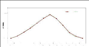
4.oe

^2.oe

7.00

6.00

^5.oe

3.oe

0.00

^1.oe

JAN FEB MAR APR MAY JUN JUL AUG SEP OCT NOV DEC

FAO Penman-Monteith - ETo
Rei. Evapotranspiration Rome

ETo (-G) ETo

f(n/N)	0.46	0.45	0.54	0.59	0.66	0.69	0.80	0.77	0.69	0.58	0.44	31.19
sigma(TxTn)	30.66	31.02	31.83	33.27	35.19	37.14	38.58	38.63	37.21	34.88	32.64	0.21
emissivity	0.21	0.21	0.21	0.20	0.18	0.17	0.16	0.16	0.16	0.18	0.19	6.46
Rbo	6.53	6.62	6.69	6.53	6.32	6.18	6.18	6.06	5.91	6.10	6.31	2.64
LWR	3.03	2.99	3.62	3.89	4.20	4.26	4.96	4.69	4.10	3.54	2.79	4.14
Rn (Rns-Rl)	4.71	6.20	8.76	11.23	13.14	13.91	14.91	13.59	11.01	7.67	5.09	-0.45
G	-0.17	0.11	0.25	0.43	0.57	0.55	0.39	0.01	-0.39	-0.66	-0.67	4.59
Rn-G	4.88	6.09	8.51	10.79	12.57	13.36	14.51	13.57	11.40	8.33	5.75	0.69
Rad Term	0.75	1.02	1.53	2.27	2.95	3.44	3.90	3.68	2.82	1.77	0.94	0.76
Rad Term(-G)	0.77	1.00	1.49	2.18	2.82	3.30	3.80	3.67	2.92	1.92	1.06	1.40
ETcomb	1.44	1.88	2.61	3.35	4.21	5.07	5.87	5.21	4.01	2.60	1.79	-5.3%
	-1.8%	1.0%	1.7%	2.6%	3.1%	2.7%	1.7%	0.1%	-2.5%	-5.8%	-6.9%	1.47
ET (-G)	1.47	1.87	2.57	3.26	4.08	4.94	5.77	5.21	4.10	2.76	1.91	13.6

APPENDIX 3: CONGO RIVER DISCHARGE DATA AT KINSHASA

Station: Kinshasa

Latitude: 4.3^o S/ Longitude: 15.3^o E River: Zaire

Country: Zaire

Elevation: m

Area: 3475000 km²

-		Jan			Feb			Mar			Apr				May			Jun			Jul			Aug				Sep			Oct			Nov			Dec			Ann
m ^3 /c		47494			37649			34713			37172				39150			36717			31703			31087				36366			43172			51708			56082			40251
mm		36.6			26.4			26.8			27.7				30.2			27.4			24.4			24				27.1			33.3			38.6			43.2			366
km 3		127			91.9			93			96.3				105			95.2			84.9			83.3				94.3			116			134			150			1270
l/s/km 2		13.7			10.8			9.99			10.7				11.3			10.6			9.12			8.95				10.5			12.4			14.9			16.1			11.6
%%		9.83			7.79			7.19			7.7				8.11			7.6			6.56			6.44				7.53			8.94			10.7			11.6			100
Year			Jan			Feb			Mar			Apr		May			Jun			Jul			Aug			Sep			Oct			Nov			Dec			Annual
1903			45250			34860			32410			32820		34970			34060			30850			31160			36900			41280			48300			51020			37823
1904			42390			34510			33760			39600		40510			36810			28700			31960			38950			45330			52340			53850			39893
1905			46230			36340			33320			33460		29970			26080			22350			24180			28120			34450			42420			49960			33907
1906			47700			37050			36550			37620		36910			34410			30660			27280			30910			40750			46980			48310			37928
1907			37680			33130			31490			31900		35110			30730			24100			23980			29390			35610			42180			45680			33415
1908			38270			30120			28350			31350		34390			33840			31320			30410			37370			44340			55350			65760			38406
1909			53560			38810			35460			42050		50530			48140			37290			36560			37940			48170			53600			54350			44705
1910			49470			39480			34890			34120		41150			37400			29960			33800			36260			44380			53550			60160			41218
1911			47110			34390			30640			34150		36560			39260			30290			26080			31460			37200			46500			55440			37423
1912			47720			38260			34750			35870		33930			30660			30930			31320			37580			46680			52490			53260			39454
1913			42280			34110			34170			34160		39650			37930			29690			27730			29040			35120			42220			40930			35586
1914			33330			26910			30320			34750		32310			31780			28950			26280			29980			40460			49340			56810			35102
1915			47450			31100			28730			29230		29470			28440			25220			25360			30420			35730			41010			47170			33278
1916			41840			31490			30370			31980		37570			32240			29100			27760			33810			43340			54960			59680			37845
1917			49120			38390			35010			37150		42470			41220			32990			29270			35990			44720			55480			55920			41477
1918			39130			29280			27900			33170		34090			29790			27440			29550			35470			37520			41500			43840			34057
1919			39500			33620			30380			30890		30240			26380			23740			26810			30550			36220			41510			44630			32873
1920			39060			30780			27230			29740		34670			32090			29370			32750			38460			42530			50110			59540			37194
1921			52780			37570			32740			32900		37460			34180			32650			30590			38200			44720			53430			55850			40256
1922			43250			36260			33300			33260		32760			29720			26750			25830			33390			41970			53000			58140			37303
1923			44370			33990			29540			34370		41650			40550			32370			33700			39390			44010			50440			59870			40354
1924			49770			38820			30880			36310		42360			41450			30620			30610			37450			44910			57970			63370			42043
1925			49950			34770			32720			34610		34580			34160			34020			32180			37050			44900			55210			64170			40693
1926			60480			40870			34900			39780		43090			38090			31770			31820			38150			44480			55730			61660			43402
1927			46500			34440			32250			38020		38370			33660			27000			27650			31860			38480			46720			47350			36858
1928			39920			34680			31430			35800		40480			42290			37830			33530			40740			45280			49460			51730			40264
1929			42270			35310			34090			34930		36640			32940			29080			30200			36110			41530			51730			57930			38563
1930			47420			37460			33870			40460		44480			40740			31160			27860			31850			40360			48210			47100			39248
1931			40220			35530			34170			36940		37550			34530			29020			28850			31750			36970			44480			49130			36595
1932			45380			32600			29860			34370		35470			38280			35610			30820			38200			46820			56200			56380			39999
1933			49740			46510			42730			42240		37350			32560			27700			28720			34020			41630			46820			50950			40081
1934			47320			33860			31090			34180		35870			33330			31160			32580			39030			43950			54800			63670			40070
1935			57310			43300			40510			43650		44760			42300			38350			31830			35580			40450			45820			49040			42742
1936			44870			37780			35270			36520		37890			35490			32900			32640			39350			47430			53580			56770			40874
1937			45880			37740			37620			40810		44140			41460			31740			31400			34770			40660			52490			57900			41384
1938	49140			34130			34410			34580			35920			32880			30100			32250			36710		42420			52350			56790			39307
1939	45860			39080			37250			38080			40880			37470			29990			29040			32020		42340			52950			62380			40612
1940	49580			41420			38640			40380			42230			38920			30210			32480			36500		42110			50240			52780			41291
1941	44440			34870			34620			35000			34180			35270			34730			31370			38020		41360			47720			57110			39058
1942	55200			45070			38440			37180			36650			36500			31190			33170			41280		46570			47860			46450			41297
1943	39330			32430			29690			30200			32200			32050			27340			28170			33840		41060			45800			43730			34653
1944	39590			35670			31670			39990			40790			36460			27090			28520			36420		43840			50270			52030			38528
1945	42080			32720			31840			31010			31360			34560			30960			30080			36830		46180			54580			56250			38204
1946	43730			31860			29340			30580			34250			31740			28120			29270			36840		46120			54850			61300			38167
1947	50350			39850			36080			39060			45990			44510			36910			34900			36730		44220			49820			49540			42330
1948	46590			39350			37990			36180			37100			35080			33560			34630			42040		50620			60170			62740			43004
1949	47360			34630			31920			33970			32800			29350			29080			32870			38140		46990			53960			51030			38508
1950	39860			33800			31250			37410			36820			32500			29480			32830			38270		45720			56940			56150			39253
1951	44720			36500			34040			41700			37730			34170			31650			28150			34240		39310			53840			62780			39903
1952	55020			38160			33000			33900			39350			38650			32250			31900			37050		43150			51020			51520			40414
1953	42748			34920			34230			35760			36900			33800			28840			25850			31910		37540			45250			49370			36427
1954	36920			29160			31780			36470			39280			35860			31830			27690			33620		40560			50180			51450			37067
1955	46760			41590			37680			41340			45350			39190			32220			32570			37440		47740			59470			60790			43512
1956	48930			38300			34460			38850			46620			41840			34750			30490			35440		42630			50390			55490			41516
1957	49770			37530			36150			44050			44230			40840			35120			32840			35380		39480			48280			54520			41516
1958	50870			37780			29820			29960			34110			30660			26130			26010			29880		35000			42100			42900			34602
1959	38510			34590			30180			30660			31260			29920			25440			25940			33870		42700			49590			57720			35865
1960	51820			40650			41510			45450			48730			43540			37560			35380			38900		46860			56680			59540			45552
1961	48220			41240			39900			42650			44510			37530			35060			36700			41410		52190			65900			80830			47178
1962	76300			61200			47280			51290			53230			48710			44760			40420			44240		52930			64320			74890			54964
1963	67950			55860			47560			47220			53230			51800			44830			39630			40690		44010			51180			58540			50208
1964	57750			47440			41830			43990			47130			46750			38790			32930			38810		47700			61390			69410			47827
1965	54640			40590			37580			43360			43370			35590			28370			30020			35980		41670			51380			62350			42075
1966	55580			43690			41880			46980			50550			47930			39300			36670			41690		48190			55550			63040			47588
1967	49130			35900			33130			35030			35220			33030			30550			31420			38050		45900			60160			65540			41088
1968	57600			44140			42800			44630			46590			46150			41570			36970			39700		43620			50420			58560			46063
1969	56690			48930			45360			52690			53070			50700			44510			43170			45980		50840			59180			66420			51462
1970	54910			44920			44300			45370			45020			42310			34480			36200			43330		51990			62820			62540			47349
1971	47930			38010			33630			35860			37540			33050			28180			32730			38690		44660			50590			54330			39600
1972	43510			34770			33130			35210			36450			33400			29580			29380			33000		36990			50140			55880			37620
1973	47060			37530			32340			32180			34650			32240			25760			26080			33170		40230			47200			50400			36570
1974	40840			34630			31530			34210			36700			35790			31530			33150			37410		44970			52150			52180			38757
1975	43490			37530			34490			34650			36450			32560			29970			29960			39110		49880			60170			63650			40993
1976	46450			38470			38300			40480			42240			38600			33940			32410			38950		44110			52040			59240			42103
1977	56190			46680			39680			43040			45650			38580			34210			33390			39260		48380			55690			57770			44877
1978	51640			37760			35800			37980			42250			41950			35860			33150			39440		44410			53640			62440			43027
1979	51920			45540			43540			45930			46870			47780			40980			33570			37600		39450			47430			52280			44408
1980	42440			35070			33340			35850			38170			37170			33780			34980			38050		45340			53790			59530			40626
1981	50000			39460			32940			36290			35540			38330			29680			30770			38900		44920			51040			52160			40003
1982	44050			35070			31400			29490			32610			34340			30680			29270			34040		41540			56690			61230			38367
1983	49020			36960			31360			31610			29980			27060			24360			25620			31250		36080			45260			47720			34690

APPENDIX 4: ATTRIBUTE TABLE FOR DRAINAGE NETWORK ORDERING

Domain	The IDs of the Table's domain, every record (ID) represents a certain stream.
UpstreamLinkID	The IDs of the streams that directly contribute to the current stream, e.g. when streams 5 and 7 flow together into stream 12, then the UpstreamLinkID column will read for the record with ID 12: {5,7}
UpstreamCoord	The XY-coordinate of the beginning of a stream segment (down-flow); these coordinates are shown as points in the third picture above. This column is a coordinate column.
UpstreamElevation	The elevation, as extracted from the DEM, at the position of the upstream coordinate. This column is a value column.
DownstreamLinkID	The ID of the stream segment into which the current stream will flow (down-flow). This column is a value column.
DownstreamCoord	The XY-coordinate of the end of a stream segment (down-flow).
DownstreamElevation	A column containing the elevation, as extracted from the DEM, at the position of the downstream coordinate.
ElevationDifference	Height difference between upstream coordinate and downstream coordinate, i.e. UpstreamElevation - DownstreamElevation.
Strahler	Strahler ordering number; the Strahler ordering number for a stream is calculated as follows: when streams of equal order join each other: the Strahler ordering number of one of the streams that directly contributes to this stream + 1 is assigned; when streams of unequal order join each other: the largest Strahler ordering number of the streams that directly contribute to this stream is assigned; In other words: the Strahler order values of the UpstreamLinkIDs are found, when these order values are equal, the value is increased by 1; when these order values are unequal, the maximum value is assigned. The Strahler column is a value column.
Shreve	Shreve ordering number; the Shreve ordering number for a stream is calculated as the sum of the Shreve ordering numbers of the streams that directly contribute to this stream, i.e. the sum of the Shreve order values of the UpstreamLinkIDs. The Shreve column is a value column.
Length	The length of a stream measured along the drainage.
StraightLength	The length of a stream calculated as the difference between the upstream coordinate and the downstream coordinate, i.e. | UpstreamCoord - DownstreamCoord |
SlopeAlongDrainage%	The average slope in percentages between the upstream coordinate and the downstream coordinate, when the length is measured along the drainage, i.e. (ElevationDifference/Length)* 100%
SlopeAlongDrainageDegree	The average slope angle in degrees between the upstream coordinate and the downstream coordinate, when the length is measured along the drainage, i.e. tan- 1(ElevationDifference/Length)
SlopeDrainageStraight%	The average slope in percentages between the upstream coordinate and the downstream coordinate, when the length is the straight length between the upstream coordinate and the downstream coordinate, i.e. (ElevationDifference/StraightLength)* 100%
SlopeDrainageStraightDegree	The average slope angle in degrees between the upstream coordinate and the downstream coordinate, when the length is the straight length between the upstream coordinate and the downstream coordinate, i.e. tan1(ElevationDifference/StraightLength)
Sinuosity	A measure for meandering of the stream, i.e. Length / StraightLength
TotalUpstreamAlongDrainageLength	The total length of all (upstream) streams that contribute to the current stream
StrahlerClass	An additional class column to be able to display the Strahler ordering numbers as classes.

APPENDIX 5: HORTON STATISTICS FUNCTIONALITY: DEFINITION OF PARAMETERS

The Horton Statistics operation calculates for all streams with a certain (Strahler) stream order number i, located in merged catchment C with ID x:

Cx_N: the number of streams for catchment x, or The number of streams with a certain Strahler stream order number

Cx_L: the average stream length (km), or The average length (km) of the streams with this Strahler order number.

Cx_A: the average area of catchments (km²) or The average area (km²) of the catchments belonging to the streams with this Strahler order number.

Cx_N_LSq: expected values for Cx_N by means of a least squares fit through Cx_N, or The expected number of streams with a certain Strahler stream order number.

Cx_L_LSq: expected values for Cx_L by means of a least squares fit through Cx_L, or The expected average length (km) of the streams with this Strahler order number.

Cx_A_LSq: expected values for Cx_A by means of a least squares fit through Cx_A, or The expected average area (km²) of the catchments belonging to the streams with this Strahler order number.

APPENDIX 6: HORTON MORPHOLOGICAL PARAMETERS AND STATISTICS FOR SUBSEQUENT STRAHLER ORDER

	strahler Order	HORTON MORPHOLOGICAL PARAMETERS
		Calculated			Expected
		C_N	C_L	C_A	C_N_LSq	C1_L_LSq	C_A_LSq
1	1	30	64.74	3322.57	25.751	69.607	4205.716
	2	6	196.02	21035.86	8.143	169.59	14619.42
	3	3	384.32	49761.68	2.575	413.19	50818.28
	4	1	662.01	158672.2	0.814	1006.7	176648.5
	5						1
	6						1
	7						1
2	1	26	64.76	3258.19	30.213	76.663	2964.718
	2	8	183.8	14855.7	5.925	131.139	17944.58
	3	1	189.49	119366.6	1.162	224.328	108613.4
	4	1	664.74	132257.5	0.228	383.737	657405.5
	5
	6
	7
3	1	118	65.19	3137.12	133.107	80.73	3510.212
	2	32	191.43	15777.09	33.277	178.149	15224.16
	3	9	340.46	61493.83	8.32	393.127	66028.79
	4	2	932.09	296725.4	2.08	867.528	286373.8
	5	1	2130.4	646792.4	0.52	1914.403	1242034
	6
	7
4	1	168	77.44	2986.6	107.066	160.972	5432.712
	2	42	234.59	16796.23	39.039	263.615	17644.8
	3	13	476.94	63232.86	14.235	431.708	57308.19
	4	5	821.84	177175	5.19	706.985	186130.1
	5	2	1013.09	450879.8	1.893	1157.791	604528.3
	6	1	1152.81	905331.4	0.69	1896.051	1963436
	7
5	1	261	57.51	2591.04	236.501	75.237	3126.151
	2	54	185.49	16541.88	55.742	173.055	14315.61
	3	14	346.48	70292.39	13.138	398.046	65555.63
	4	3	981.2	358082.7	3.097	915.553	300199.5
	5	1	2265.76	1121600	0.73	2105.879	1374707
	6				0.172	4843.768	6295207
	7						1
6	1	151	63.27	3080.17	25.159	195.664	27871.48
	2	26	297.12	27360.17	12.592	312.666	57809.6
	3	6	589.78	129887.4	6.302	499.632	119905.7
	4	1	605.16	779475.3	3.154	798.399	248702.4
	5	1	1655.82	823385.2	1.578	1275.822	515845.9
	6	2	1847.5	417141.4	0.79	2038.731	1069941
	7	1	2445.2	859575.2	0.395	3257.842	2219218

APPENDIX 7 PEARSON PRODUCT MOMENT CORRELATION BETWEEN
HORTON AND GIUH

Friday, June 27, 2008, 3:52:27 AM
Data source: Data 1 in Notebook 1

Pearson Product Moment Correlation Friday, June 27, 2008, 3:52:27 AM

Data source: Data 1 in Notebook 1

Cell Contents:

Correlation Coefficient

P Value Number of

Samples

	Rb	Rl	Ra	LHSOr	Tpg	Qpg	Tpg
Rb		0.903	0.952	-0.284	-0.464	0.504	-0.464
		0.0137	0.00345	0.585	0.354	0.308	0.354
		6	6	6	6	6	6
Rl			0.958	-0.287	-0.494	0.532	-0.494
			0.00267	0.582	0.32	0.277	0.32
			6	6	6	6	6
Ra				-0.386	-0.586	0.598	-0.586
				0.45	0.222	0.209	0.222
				6	6	6	6
LHSOr					0.965	-0.96	0.965
					0.00182	0.00243	0.00182
					6	6	6
Tpg						-0.975	1
						0.000899	0
						6	6
Qpg							-0.975
							0.000899
							6

APPENDIX 8.a. LOCAL WATER BALANCE FOR SELECTED GRID CELLS IN THE CONGO RIVER BASIN (TABLE)

PPT = Precipitation, PEH= Effective Precipitation, PET= Potential Evapotranspiration, AET = Actual Evapotranspiration, SOM= Soil Moisture, ROF= Runoff, C= Vertical Integrated Moisture Convergence

Long Lat		Item	Dec Jan Feb Mar Apr May Jun Jul Aug Sep Oct Nov DJF MAM JJA SON																Ann.
18.31	4.24	AET	32.2	18.8	34.6	89.3	106.5	121.2	102.3	102.5	102.5	105.2	105.6	91.3	85.5	317.1	307.2	302.1	1011.9
18.31	4.24	PET	114.7	117.9	117.8	136.4	128.8	121.0	102.2	102.4	102.4	105.2	105.8	105.2	350.5	386.2	307.0	316.2	1359.8
18.31	4.24	PPT	31.3	20.4	37.5	108.9	137.1	170.8	140.0	178.4	227.3	192.8	195.6	92.6	89.3	416.8	545.7	480.9	1532.7
18.31	4.24	ROF	1.2	0.4	0.1	0.0	0.0	0.0	0.0	11.8	33.2	29.3	13.7	4.1	1.7	0.0	45.0	47.1	93.9
18.31	4.24	SOM	0.0	0.0	0.0	0.0	0.0	2.9	9.3	17.6	17.6	17.6	17.6	3.9	0.0	2.9	44.5	39.1	86.6
18.31	4.24	C	-0.1	0.0	0.0	0.0	0.0	0.1	0.2	0.7	1.1	1.0	0.4	-0.3	-0.1	0.1	1.9	1.1	3.1
21.04	-0.04	AET	105.8	108.7	108.3	122.3	112.5	110.2	100.1	96.2	105.1	107.8	110.1	103.5	322.8	345.0	301.3	321.4	1290.5
21.04	-0.04	PET	105.8	113.8	113.6	122.3	112.5	110.2	100.1	96.2	105.1	107.8	110.1	103.5	333.2	345.0	301.3	321.4	1300.9
21.04	-0.04	PPT	165.0	123.3	135.7	181.5	159.0	189.1	143.1	146.5	184.7	192.2	233.7	210.9	424.0	529.6	474.3	636.8	2064.7
21.04	-0.04	ROF	7.4	2.2	0.7	0.2	0.1	0.0	0.0	0.0	0.0	8.0	23.4	24.5	10.2	0.3	0.0	55.9	66.4
21.04	-0.04	SOM	17.6	7.4	4.7	10.9	16.6	17.6	17.6	17.6	17.6	17.6	17.6	17.6	29.7	45.1	52.8	52.8	180.4
21.04	-0.04	C	0.1	-0.3	-0.1	0.2	0.2	0.5	0.4	0.5	0.7	0.8	1.0	1.2	-0.2	0.9	1.6	3.0	5.2
28.52	-2.31	PET	115.2	122.4	118.4	136.3	123.4	119.8	103.5	100.9	103.5	109.8	111.6	107.2	356.0	379.5	307.9	328.5	1371.9
28.52	-2.31	PPT	165.4	136.1	133.8	181.2	170.2	107.1	32.4	16.6	57.3	105.9	134.9	175.5	435.3	458.4	106.3	416.3	1416.4
28.52	-2.31	ROF	1.2	0.4	0.1	0.0	0.0	0.0	1.8	14.9	29.2	21.7	13.0	3.9	1.6	0.0	45.9	38.6	86.2
28.52	-2.31	SOM	1.2	0.0	0.0	0.0	0.0	11.3	28.2	28.2	28.2	28.2	28.2	17.4	1.2	11.3	84.5	73.7	170.6
28.52	-2.3 1	C	0.9	0.5	0.6	0.9	0.9	0.0	-0.4	0.0	0.0	0.0	0.3	1.0	2.0	1.8	-0.4	1.2	4.6
28.52	-2.30	AET	95.2	100.5	93.6	102.9	92.9	91.0	41.3	16.7	51.4	86.6	99.7	97.5	289.2	286.9	109.4	283.8	969.4
22.25	-5.56	AET	112.0	114.6	109.7	122.9	110.8	87.7	12.3	7.6	19.8	65.2	122.1	106.5	336.3	321.4	39.8	293.9	991.4
22.25	-5.56	PET	108.7	111.7	103.6	114.9	108.2	118.1	114.5	112.2	112.1	114.4	124.4	111.3	324.1	341.2	338.8	350.1	1354.2
22.25	-5.56	PPT	232.2	137.5	125.6	204.4	177.5	76.5	17.6	15.6	49.6	126.5	171.6	235.3	495.3	458.3	82.7	533.4	1569.7
22.25	-5.56	ROF	0.0	0.0	0.0	0.0	1.4	0.4	0.1	0.0	0.0	0.0	0.0	0.0	0.0	1.8	0.2	0.0	2.0
22.25	-5.56	SOM	28.2	23.6	20.9	28.2	28.2	4.7	0.1	0.0	0.0	0.0	0.4	28.2	72.7	61.0	0.2	28.6	162.4
22.25	-5.56	C	0.9	0.1	0.0	0.6	0.1	-0.7	-0.1	0.0	0.0	0.0	0.0	1.1	1.0	0.0	-0.1	1.1	2.0
15.22	-4.22	AET	105.5	109.8	107.2	122.2	114.1	105.4	25.8	2.8	3.6	35.9	98.4	107.8	322.6	341.6	32.1	242.1	938.4
15.22	-4.22	PET	105.5	109.8	109.4	122.2	114.1	106.0	90.5	93.6	106.7	113.8	116.0	107.8	324.8	342.2	290.9	337.7	1295.6
15.22	-4.22	PPT	162.8	142.4	121.1	180.9	213.7	125.1	4.5	1.8	3.5	38.6	123.6	246.2	426.2	519.8	9.7	408.4	1364.2
15.22	-4.22	ROF	13.1	4.1	1.2	0.4	8.4	2.5	0.8	0.2	0.1	0.0	0.0	8.5	18.4	11.3	1.0	8.5	39.2
15.22	-4.22	SOM	27.7	27.7	18.1	24.2	27.7	22.2	1.0	0.0	0.0	0.0	0.0	27.7	73.6	74.1	1.0	27.7	176.5
15.22	-4.22	C	0.4	0.1	-0.3	0.2	0.4	-0.1	-0.7	0.0	0.0	0.0	0.0	1.2	0.3	0.5	-0.7	1.2	1.3
25.11	0.31	AET	101.2	82.1	88.8	119.3	112.3	108.6	94.5	79.5	98.5	102.1	108.9	101.9	272.1	340.2	272.5	312.9	1197.7
25.11	0.31	PET	108.4	114.6	114.7	123.8	116.8	111.6	96.2	96.0	99.1	108.0	114.5	107.9	337.8	352.1	291.3	330.3	1311.5
25.11	0.31	PPT	101.7	71.5	96.2	164.0	179.1	161.7	109.2	119.5	156.0	184.9	214.1	196.3	269.4	504.8	384.7	595.4	1754.2
25.11	0.31	ROF	7.8	2.3	0.7	0.2	0.6	1.5	0.4	3.3	11.6	16.8	24.6	25.9	10.8	2.3	15.3	67.3	95.7
25.11	0.31	SOM	4.7	0.3	0.0	0.0	11.2	17.0	11.8	12.3	17.6	17.6	17.6	17.6	5.0	28.3	41.7	52.8	127.8
25.11	0.31	C	-0.2	-0.1	0.0	0.0	0.4	0.2	-0.2	0.0	0.5	0.6	0.8	0.9	-0.2	0.6	0.3	2.2	2.9
27.29	-11.40	AET	109.6	112.4	104.4	106.2	99.1	17.0	0.2	0.0	1.3	20.1	78.2	112.1	326.3	222.4	1.5	210.4	760.5
27.29	-11.40	PET	113.3	111.6	98.0	117.1	118.7	119.7	108.5	118.4	142.4	163.4	175.5	135.3	322.9	355.4	369.3	474.2	1521.9
27.29	-11.40	PPT	259.2	247.5	267.6	206.0	55.9	2.6	1.0	1.6	0.0	2.1	33.6	164.2	774.3	264.6	2.6	200.0	1241.5
27.29	-11.40	ROF	12.7	23.8	24.3	12.0	3.6	1.1	0.3	0.1	0.0	0.0	0.0	0.0	60.7	16.7	0.5	0.0	77.9
27.29	-11.40	SOM	28.2	28.2	28.2	28.2	2.5	0.0	0.0	0.0	0.0	0.0	0.0	0.0	84.5	30.7	0.0	0.0	115.2
27.29	-11.40	C	1.1	0.9	1.6	0.2	-0.8	-0.1	0.0	0.0	0.0	0.0	0.0	0.0	3.6	-0.7	0.0	0.0	2.9
16.03	1.37	AET	81.0	55.8	81.2	111.7	105.0	102.3	87.1	86.6	93.0	99.0	105.4	99.0	218.0	319.0	266.7	303.4	1107.1
16.03	1.37	PET	105.4	99.3	98.1	111.7	105.0	102.3	87.1	89.9	93.0	99.0	105.4	99.0	302.7	319.0	270.0	303.4	1195.2
16.03	1.37	PPT	74.2	60.3	96.1	151.0	134.3	179.0	143.7	91.7	144.0	223.0	237.1	172.1	230.6	464.3	379.3	632.1	1706.3
16.03	1.37	ROF	9.0	2.7	0.8	0.2	0.1	8.1	10.5	3.1	7.4	33.0	39.0	29.9	12.5	8.4	20.9	102.0	143.8
16.03	1.37	SOM	1.8	0.1	0.1	3.4	3.5	17.6	17.6	8.8	17.6	17.6	17.6	17.6	2.0	24.5	44.1	52.9	123.5
16.03	1.37	C	-0.2	0.0	0.0	0.1	0.0	0.7	0.3	-0.2	0.5	1.1	1.3	1.0	-0.2	0.8	0.7	3.4	4.7
20.04	-11.04	AET	114.2	115.8	107.6	109.9	101.8	18.3	0.0	-0.1	2.6	23.5	78.7	117.2	337.6	229.9	2.5	219.4	789.4
20.04	-11.04	PET	114.2	115.8	107.6	109.9	110.9	122.0	113.3	125.5	144.0	148.1	140.2	117.2	337.6	342.8	382.8	405.5	1468.6
20.04	-11.04	PPT	214.3	212.3	182.1	205.0	101.1	7.2	-0.2	-0.2	2.6	24.9	92.1	172.3	608.6	313.3	2.2	289.3	1213.4
20.04	-11.04	ROF	4.1	18.5	20.3	9.4	2.8	0.8	0.3	0.1	0.0	0.0	0.0	0.0	42.9	13.1	0.4	0.0	56.3
20.04	-11.04	SOM	28.2	28.2	28.2	11.1	0.2	0.0	0.0	0.0	0.0	0.0	7.3	21.2	84.5	11.3	0.0	28.5	124.3
20.04	-11.04	C	0.8	0.6	0.7	0.3	-0.5	-0.3	0.0	0.0	0.0	0.0	0.0	0.2	2.1	-0.5	0.0	0.2	1.9
23.05	8.00	AET	4.5	0.8	7.0	51.5	88.7	123.5	113.4	103.4	108.0	109.7	116.9	43.6	12.3	263.7	324.8	270.2	871.0
23.05	8.00	PET	114.2	114.6	99.7	112.7	110.1	123.6	128.4	133.2	136.1	131.7	136.6	121.3	328.5	346.4	397.7	389.6	1462.1
23.05	8.00	PPT	258.2	195.3	188.0	232.0	181.6	48.5	3.5	0.5	18.8	81.6	161.4	242.9	641.5	462.0	22.7	486.0	1612.2
23.05	8.00	ROF	8.8	8.2	12.0	8.5	2.5	0.8	0.2	0.1	0.0	0.0	0.0	0.0	29.1	11.7	0.3	0.0	41.2
23.05	8.00	SOM	28.2	28.2	28.2	28.2	28.2	1.6	0.0	0.0	0.0	0.0	0.0	26.6	84.5	58.0	0.0	26.6	169.0
23.05	8.00	C	0.8	0.7	1.0	1.0	0.0	-0.8	-0.1	0.0	0.0	0.0	0.0	0.9	2.5	0.2	-0.1	0.9	3.6
32.03	-5.05	AET	113.1	114.6	107.9	125.2	119.0	79.7	17.7	8.3	59.4	95.5	124.4	115.3	335.7	324.0	85.3	335.3	1080.3
32.03	-5.05	PET	116.9	116.0	110.8	123.0	118.8	126.5	129.4	143.0	158.8	158.8	159.8	122.9	343.7	368.4	431.2	441.5	1584.8
32.03	-5.05	PPT	164.1	127.6	121.8	152.5	168.9	55.1	4.2	0.0	-0.1	12.5	46.0	130.7	413.6	376.4	4.2	189.2	983.3
32.03	-5.05	ROF	25.3	10.0	5.0	15.6	3.5	1.0	0.3	0.1	0.0	0.0	0.0	6.5	40.3	20.2	0.4	6.5	67.4
32.03	-5.05	SOM	-5.1	5.2	2.1	0.9	0.6	12.2	0.1	0.0	0.0	0.0	0.0	0.0	2.3	13.6	0.1	0.0	16.0
32.03	-5.05	C	0.1	0.0	0.0	0.0	0.1	0.0	0.0	0.0	0.0	0.0	0.0	0.0	0.1	0.1	0.0	0.0	0.2

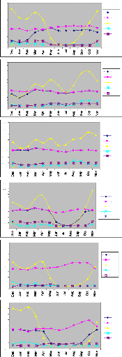
300

260

220

300

260

220

300

260

220

300

260

220

300

260

220

300

260

220

180

140

100

180

140

100

180

140

100

180

140

100

180

140

100

180

140

100

-20

-20

-20

-20

-20

-20

60

20

60

20

60

20

60

20

60

20

60

20

LUBUMBASHI(-14, 27)

UP-NORTH

BOYENDE

URAMBO

KINSHASA

OUESSO

AET PET PPT ROF SOM

AET PET PPT ROF SOM

AET PET PPT ROF SOM

AET PET PPT ROF SOM

AET PET PPT ROF SOM

AET PET PPT ROF SOM

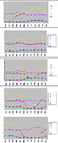
300

260

220

300

260

220

300

260

220

300

260

220

180

140

100

180

140

100

300

260

220

180

140

100

180

140

100

180

140

100

-20

-20

-20

-20

20

60

20

60

20

60

20

60

20

60

20

BUKAVU (28.52, -2.30)

SOUTH-WEST

KANANGA

BANGUI

KISANGANI

AET PET PPT ROF SOM

AET PET PPT ROF SOM

AET PET PPT ROF SOM

AET PET PPT ROF SOM

AET PET PPT ROF SOM

APPENDIX 8.b. LOCAL WATER BALANCE FOR SELECTED GRID CELLS IN THE CONGO RIVER BASIN (GRAPHS)

APPENDIX 9: SEASONAL DISTRIBUTION OF THE CONVERGENCE MOISTURE SAMPLES FOR SELECTED GRID CELLES OVER THE CONGO BASIN (C)

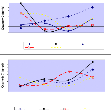
4

3

3

2

2

1

1

0

-1

-1

DJF MAM JJA SON

BOYENDE LUBUMBASHI KINSHASA

SOUTH-WEST BUKAVU

4

3

3

2

2

1

1

0

-1

-1

DJF MAM JJA SON

KISANGANI OUESSO BANGUI UP-NORTH

The first graph shows stations in the southern hemisphere. The second corresponds to the northern hemisphere.