Memoire Online - Monetary Policy Strategy in Rwanda

Submitted in partial fulfillment of the requirements for the Master's degree of commerce (Economics).

I declare that this is my own work, except where acknowledged in the text, and has been submitted or a degree at any other university.

DECLARATION.....................................................................................i

TABLE OF CONTENTS...........................................................................ii

LISTE OF TABLES.................................................................................iv

LISTE OF FIGURES................................................................................v

DEDICATION.......................................................................................vi

AKNOWLEDGEMENTS.........................................................................vii

ABSTRACT........................................................................................viii

Chapter 1: INTRODUCTION..................................................................... 1

2.1: Objective of monetary policy.................................................................5

2.2: The instruments of monetary policy.........................................................7

2.3: Monetary policy strategies....................................................... ............10

2.3.1: Choosing and using a target............................................................... 11

2.3.2: Monetary policy rules...................................................................... 12

2.3.2.1: Exchange rate rule........................................................................13

2.3.2.2: Money supply rule........................................................................14

2.3.2.3: Nominal GDP target rule.................................................................16

2.3.2.4: Inflation targeting rule....................................................................18

2.3.2.5: Taylor rule.................................................................................21

Chapter 3: MONETARY POLICY IN RWANDA.............................................23

3.1: Macroeconomic background.................................................................23

3.2: Monetary and exchange rate policy management.........................................25

3.2.1: Monetary policy.............................................................................26

3.2.2: Exchange rate policy........................................................................29

BY MEANS OF MODEL.........................................................................31

4.1: Empirical analysis.............................................................................34

4.1.1: Reaction function for Rwanda.............................................................34

4.1.2: Methodology..................................................................................36

4.1.2.1: Data...........................................................................................36

4.1.2.2 Time series properties of the data........................................................37

4.2: Estimation results..............................................................................40

SUGGESTION.........................................................................47

BIBLIOGRAPHY..................................................................................49

APPENDIX..........................................................................................54

Inflation observed in percentage...................................................................................27

Net Interior Asset (NIA)In percentage.........................................................29

Table 4.1 Unit root test-levels of variables................................................... 38

Table 4.2 Unit root tests of the first difference............................................... 38

estimation of equation 4................................................ .........................40

Estimation of equation 5.........................................................................42

M2 and inflation:1997-2002............................................................................28

My thanks goes to my academic supervisor Dr Nicola Viegi for his guidance, inspiration, comments and criticism which inspired many ideas and produced some very satisfying solutions.

I have profound gratitude to Professor Rwigamba Balinda, the Rector of Kigali Independent University, for sponsoring my post graduate studies at the University of Kwazulu-Natal.

Thanks goes to my friends and colleagues in the economic department for making my student life enjoyable.

Thanks also goes to my family and all friends for their encouragement and support which they have given me during my studies.

Last but not least, special thanks goes to my Lord Jesus Christ for all the Blessings, which, I enjoy in this life.

ABSTRACT

The aim of this dissertation is to study how monetary policy is conducted in Rwanda. The task has been accomplished by designing and estimating a Taylor rule, monetary policy reaction function for the National Bank of Rwanda over the period 1997-2001.

Applying Ordinary Least Squared (OLS) on the time series data, we test whether the Central Bank in Rwanda reacts to changes in the inflation gap, the output gap and the exchange rate. The results of the study show that the Central Bank of Rwanda has had a monetary policy over the years with the monetary stock aggregate (M1) as the principal instrument. The results also show that the Central Bank of Rwanda reacted by giving much importance to the exchange rate than to inflation and neglected the output.

In recent years, Central Banks appear to have conducted prudent monetary policies in several countries. In such a context, the role of monetary policy as a stabilisation policy is becoming more powerful and well determined. As argued in Blinder (1998), Central Banks have never been more powerful than now. Monetary policy has become the principal means of macroeconomic stabilisation, and in most countries it is entrusted with the responsibility of an independent Central Bank.

From the experience of developed economies in the world which exhibit strong economic management, various countries in developing economies have undertaken economic reforms consisting essentially of a set of market-oriented economic policies intended to readjust the economy to the liberalisation as well as bringing about an institutional reorganisation.

In the sub-Sahara African context, reforms increased significantly in the 1990s. The broad strategy has been the emphasis placed on the policy programs supported by the International Monetary Fund (IMF) and the World Bank, including among others fiscal reforms, liberation of exchange restriction and the adoption of indirect instrument of monetary policy, market-based interest policies, and so on. (IMF, December 2000).

Rwanda is no exception to this situation. Rwanda's economy is very small and open, heavily reliant on the export of few major products, especially coffee and tea. In addition it is also very reliant on imports for most of its consumables.

The destruction of the economic base that took place during the civil war period (1990-1994) forced the authorities to begin a process of economic liberalisation: to turn away from the situation of control, regulation and state command and turn towards more market related policies since 1994. In 1997, Rwanda embarked on a program of sustainable economic growth. A revised Central Bank statute underpinning the National Bank of Rwanda's independence in conducting the country's monetary policy was adopted. The period of 1998/99-2000/2001 was characterized by an enhanced structural adjustment facility program supported by IMF and World Bank. Based on this strategy, the macroeconomic objectives included an annual average real Gross Domestic Product (GDP) growth of 8 percent a year during the period 1998-2000; and a reduction in inflation to 5 percent by end 1999. In the period 1999-2002, the macroeconomic objectives were to achieve an annual real GDP growth of 6%, while keeping inflation at or below 3%.

In such program, the monetary policy played a central role in producing macroeconomic stability. It stated that monetary and credit policies would aim at further reducing the rate of inflation, and the authorities would continue to monitor development in both reserve money and broad money closely (IMF and Rwanda 1995/2002).

What it is clear from the Rwandan Central Bank behavior is that an achievement of the inflation target seems to be a fundamental goal of the monetary authority. On the basis of all the macroeconomic objectives mentioned above, Rwandan monetary authorities seem to assess the performance of monetary policy rules in terms of their effect on inflation and output. Such an assessment can be based on a situation in which the Central Bank refers to an equation, which is intended to establish the goal that has actually been influencing the actions of the Central Bank. One could interpret such behavior as being approximated by a particular rule referred to as the Taylor rule. In such a rule, monetary policy is adjusted in response to the deviation of inflation from its target value and the deviation of output from potential.

More than five years have passed since the monetary policy was given a central role in maintaining macroeconomic stability and a new statute has provided rule for monetary policy objectives and Central Bank independence. Enough observations have become available to perform an assessment of the Rwanda Central Bank's conduct of monetary policy based on choosing a rule and then using a model of the economy to examine how the economy would have behaved under the rule.

The objective of the thesis is thus, to attempt to approximate the policy behavior of the Rwanda Central Bank by estimating a variant of the Taylor rule for Rwanda. In this specific model, the dependent variable is the monetary base that the Central Bank is assumed to control, while the explanatory variables are those that are assumed to affect Rwanda Central Bank's behavior. By attempting to measure the policy behavior, the question that arises is what was the Central Bank really reacting to? Or in other words, which targets did the Central bank actually follow?

- Review the literature on the theoretical foundation of monetary policy: examining the process of monetary policy and describing monetary policy strategies

- Describe the monetary policy strategy in Rwanda by means of a model. That is, a Taylor Rule monetary policy reaction function applied to Rwanda and to interpret the estimated results in the context of the Rwandan economy.

The Taylor Rule has been considered as a representation of Central Bank behavior in various countries. It provides information about the responsiveness of the monetary policy instrument to the monetary variables. Therefore, estimating the policy behavior of the Rwanda Central Bank and determining the target the Central Bank followed, is essential to the different policy implications, especially to the implementation of an accurate and successful monetary policy.

Chapter 1 is an introduction. Chapter 2 presents the theoretical foundation of monetary policy and describes the process of monetary policy and monetary policy strategies focusing on the discussion about the main rules for monetary policy. Chapter 3 presents the monetary policy in Rwanda and describes the way the National Bank of Rwanda formulates and carries out its monetary policy. It also shows exchange policy management and its relationship to the monetary policy. Chapter 4 presents an illustration of the monetary policy strategy by means of a model and focuses on estimating a Taylor-type monetary reaction function for Rwanda. This chapter also covers the methodology, including the estimation results and its analysis. Finally in chapter 5, a conclusion and suggestion are provided.

2.1 THE OBJECTIVES OF MONETARY POLICY

Broadly speaking, the objective of monetary policy is to influence the performance of the economy as reflected in factors such as inflation, economic output and employment. It works by affecting demand across the economy in terms of people and firms willingness to spend on good and services (Federal Reserve Bank of San Francisco, 2004).

In such context, the main goal of any monetary policy is to maintain stability in the broadest sense. Wallich (1982: 45) explained that by helping to promote price stability and to avoid recession monetary policy contributes to a framework within which the market can operate with greater confidence. According to Mishkin (1997) six basic goals are continually mentioned by Central Banks when they discuss the objective of monetary policy:

In general, a high employment level has a strong link with a sustainable output and this relationship makes the employment an important objective. Indeed, it can be considered that when unemployment is high, resources and workers are not sufficiently used in the economy and this results in a low output.

The goal of economic growth is related to the one of employment. Indeed, the economy is characterised by business cycles in which output and employment are above or below their long term levels. The role of monetary policy consists of affecting the output and the employment in the short term. For example, when demand weakens and there is a recession, the Central Bank can stimulate the economy temporarily and help push it back toward its long term level of output by lowering interest rates.

The goal of price stability is also most desirable. This can just be illustrated by the fact that persistent attempts to expand the economy beyond its long term growth path will result in capacity constraints and will lead to higher inflation without lowering unemployment or increasing output in the long term (Federal Reserve Bank of San Francisco, 2004). Dornbusch, Fisher and Startz (2001) show in the same way how the costs of high inflation are easy to see: in countries where prices increase all the time, money no longer a useful medium of exchange, and sometimes output drops dramatically.

According to Mishkin (1997: 476), the goal of interest-rate stability, stability of financial markets and stability in foreign exchange markets can be shown in short as the following:

Interest- rate stability is important because fluctuations in interest rates can lead to uncertainty in the economic environment and disrupt the plan for the future. Concerning the stability of financial markets, it is known that financial crises can interfere with the ability of financial markets to channel funds to people with productive investment opportunities, resulting in a sharp reduction in economic activity. Having a stable financial system in which financial crises are avoided is an important goal for a Central Bank.

Finally, the stability in foreign exchange markets has become a major consideration of the Central Bank given the increase in international trade and the increase in international integration.

Not all of those goals can be pursued by a given Central Bank. Each one has to choose which goals they consider most important and vital to their economic realities. However, when Central Banks have to decide about which specific objectives to adopt, some conflicts among goals create veritable difficulties. Mishkin (1997) explains that although many of the goals mentioned are consistent with each other, this is not always the case. The goal of price stability often conflicts with the goals of interest-rate stability and high employment in the short term.

When all these bank's objectives are decided upon, the next question becomes what instruments or tools does the Central Bank need to put into operation and how useful are these tools?

2.2 THE INSTRUMENTS OF MONETARY POLICY

After selecting monetary policy objectives, Central Banks make use of various monetary policy instruments at their disposal. Fundamentally these instruments allow the Central Bank to stimulate or slow down the economy by influencing the quantity of money and credit the banks can provide to their customers through loans. Two types of monetary instruments are generally classified, namely indirect and direct policy.

According Gidlow (1998), the indirect policies are considered to be actions taken by the Central Bank whereby it achieves its monetary policy aims by encouraging market participants to take particular actions in terms of their lending and borrowing behavior. These actions may be the result of price and interest rate incentives or disincentives brought about in the financial market. The direct policy instruments on the other hand refer to the measures taken by Central Bank that seek to attain the aims of monetary policy by means of certain rules prescribing the behavior pattern of banks and possibly other financial institutions. The indirect instrument is also considered as market-oriented whereas the direct instrument is a non-market-oriented. Meyer (1980) agreed that monetary policy instruments are generally classified as either general or selective controls. General controls have their primary effect on either the net monetary base or the size of the money multiplier. These include open market operations, changes in reserve requirements, and changes in the discount rate. Selective controls on the other hand, have their primary influence on the allocation of credit among alternative uses. The examples of selective controls include margin (or down payment) requirements for loans to acquire securities and interest rate ceilings on rates paid by banks on savings accounts or charged by banks on loans. Gidlow (1998) provided as an example of direct policy instruments, the case of instructions sent to banks under which the latter are requested not to exceed a certain amount of lending to domestic private sector borrowers as specified period, and instructions that banks must not quote interest rates above or below a certain maximum or minimum level on their various credit and deposit facilities made available to customers. Alexander et al (1995:14) also provided an interesting explanation about direct and indirect policy instruments. They showed that the term «direct» refers to the one- to one correspondence between the instrument (such as credit ceiling) and the policy objective (such as a specific amount of domestic credit outstanding). Direct instruments operate by setting or limiting either prices (interest rates) or quantities (amounts of credit outstanding) through regulations, while indirect instruments act on the market by, in the first instance, adjusting the underlying demand for, and supply of bank reserves. Based on these descriptions, it can be noted that both types of policy instruments play an important role in economic activities. However, direct and indirect instruments do not have the same effectiveness in improving market efficiency in the same economic environment. As has been specified previously, the most common direct instruments are interest rate controls, credit ceilings and directed lending. Alexander et al (1995: 15) argued that «direct instruments are perceived to be reliable, at least initially in controlling credit aggregates or both the distribution and the cost of credit. They are relatively easy to implement and explain and their direct fiscal costs are relatively low. They are attractive to governments that want to channel credit to meet specific objectives». In countries with very rudimentary and noncompetive financial systems, direct controls may be the only option until the institutional framework for indirect instruments has been developed. The same authors also showed the disadvantages of direct instruments. These consist of the fact that credit ceilings are based on amounts extended by particular institutions and therefore they tend to ossify the distribution of credit and limit competition, including the entry of new banks. All those advantages lead to the conclusion that direct instruments often lose their effectiveness because economic agents find means to circumvent them.

The open market operations are often seen as the most important monetary policy tool because they are the primary determinants of changes in interest rates and the monetary base and are the main source of fluctuations in the money supply (Mishkin, 1997).

The way this instrument influences the economy can be seen from purchase or sale of financial instruments by the Central Bank. Open market purchases expand the monetary base, thereby raising the money supply and lowering the short-term interest rates. Conversely, open market sales reduce the reserves of the banking system, reducing the ability of banks to lend and invest, and limiting the amount of funds available for the economy to use (Federal Reserve System and Monetary Policy, 1979).

Open market operations are also based upon dynamic defensive operations; dynamic operations are those taken to increase or decrease the volume of reserves in order to ease or tighten credit. Defensive operations, on the other hand, are those taken to offset the effects of other factors influencing reserves and the monetary base.

Another interesting indirect monetary policy tool concerns the changes in the reserve requirements. This consists of obliging banks to hold a specified part of their portfolios in reserves at the Central Bank (Alexander et al, 1995). This instrument affects the money supply by causing the money multiplier to change.

Lastly, the Central Bank's lending facilities it is an indirect instrument, which is often well known as discount policy. The discount policy involves changes in the discount rate which affects the money supply by affecting the volume of discount loans and the monetary base. A rise in discount loans adds to the monetary base and expands the money supply whereas a fall in discount loans reduces the monetary base and shrinks the money supply (Mishkin, 1997).

Once all the instruments mentioned above are well applied, the results easily seen in the level of economic activity since those instruments influence the growth of the money supply as well as other financial variables.

However, it is also worth noting that by using indirect instruments, the Central Bank can determine the supply of reserve money in the long term only under a fully flexible exchange rate regime. Even under a pegged or managed exchange rate regime, however, Central Bank transactions affect reserve money, at least in the short term. These transactions affect bank's liquidity position, which results in adjustments to interbank, money market, and bank loan and deposit interest rates to re-equilibrate the demand for, and the supply of, reserve balances (Alexander et al, 1995).

2.3 MONETARY POLICY STRATEGIES

Having identified the instruments available for active monetary policy implementation, it is important to understand the current conduct of monetary policy. The latter needs to be operated within a well-defined independent Central Bank.This means simply to provide the authorities of Central Banks with the power to determine quantities and interest rates on its own transactions without interference from government institutions (Lybeck, 1998 quoted in Worrel, 2000). Similarly, Blinder (1998) shows that Central Bank independence means two things: Firstly, that the Central Bank has the freedom to decide how to pursue its goals, and secondly, that its decisions are very difficult for other branches of government to reverse. This implies that an independent Central Bank needs to be free of the political pressures that influence other government institutions. This is particularly important when a Central Bank needs to target inflation, exchange rates or the monetary base for example. On this basis, an important point to analyse could be the way Central Banks process before following a given strategy.

2.3.1 Choosing and Using a Target

As is already known, in conducting monetary policy, Central Banks have the responsibility to achieve certain goals or final objectives. The latter could be the inflation rate, the GDP and others. According to Mishkin (1997) the strategy can be explained as follows: «after deciding on its goals, the Central Bank chooses a set of variables to aim for called intermediate targets such as monetary aggregates, interest rates etc. which have a direct effect of the goals. The Central Bank's policy tools do not directly affect these intermediate targets. Alongside this, the Central Bank chooses another set of variables to aim for, called operating targets or instruments among others reserve aggregates or interest rates which are more responsive to its policy tools» (Mishkin, 1997: 478) In more general terms, Mishkin argued that the main reason for trying to achieve its goal by using intermediate and operating target, is simply to allow the Central Bank to judge whether its policies are on the right path and to make mid-course corrections, rather than waiting to see the final outcome of its policies.

The process starts from Central Bank policy tools and directly affects the operating targets, which in their turn affect the intermediate targets, and finally the latter affect the goals. As has been specified above, the intermediate targets comprise monetary aggregates and interest rates. In practice three criteria are suggested for choosing one target between them. The three criteria can be summarised briefly as follows:

- Measurability: quick and accurate measurement of an intermediate target variable is necessary because the intermediate will be useful only if it signals when policy is off track more rapidly than the goal.

- Controllability: The good intermediate target is the one on which the Central Bank must be able to exercise an effective control.

- Predictable effect on goals: the goals must have a close link with intermediate target chosen. (Mishkin, 1997:482).

The same criteria remain valid about choosing the operating targets. A preferable operating target must have a more predictable impact on the most desirable intermediate target.

The strategy described above is not, of course the only one that allows a well conducted of monetary policy. In addition, Central Banks have increasingly sought to reach their objective of macroeconomic stability through the adoption of certain principles known as rules for monetary policy.

2.3.2 Monetary Policy Rules

According to Taylor (1998) the monetary policy rule is defined as a description, expressed algebraically, numerically and graphically-of how the instruments of policy such as the monetary base or federal funds rate, change in response to economic variables. Taken in a general sense, a rule can be defined as «nothing more than a systematic decision-making process that uses information in a consistent and predictable way» (Taylor, 1998:2). The concept of monetary policy rule is the application of this principle in the implementation of monetary policy by the Central Bank (Poole, 1999). Svensson (1998) defines a monetary policy rule simply as a prescribed guide for monetary policy conduct.

In policy conducted by rule, policymakers announce in advance how the policy will respond in various situations, and commit themselves to following through. Taylor (1998) notes that one monetary policy rule can be said to be better than another monetary policy rule if it results in better economic performance according to the same criteria such as inflation or the variability of inflation and output.

In the following pages, various economic rules such as the Exchange Rate Targeting Rule, the Money Supply Rule, GDP Targeting Rule, Inflation Targeting Rule and Taylor Rule will be discussed in terms of their abilities to guide Central Bankers.

2.3.2.1 Exchange Rates Rule

Exchange rate regime considerations play a strong role in influencing monetary policy in a country. The rate of exchange means the price of one currency in comparison with another currency. Mishkin (1997) argued that «if a Central Bank does not want to see it currency fall in value, it may pursue a more contractionary monetary policy and reduce the money supply to raise the domestic interest rate, thereby strengthening its currency. Similarly if a country experiences an appreciation in its currency, domestic industries may suffer from increased foreign competition and may pressure the Central Bank to pursue a higher rate of monetary growth in order to lower the exchange rate» (Mishkin, 1997: 523).

The two most noted exchange rates regimes, fixed and floating exchange rates tend to be extended from pegs to target zones, to floats with heavy, light, or no intervention.

Initially, in a fixed exchange rate system, the exchange rates are determined by the governments and Central Banks rather than the free market, and are maintained through foreign exchange market intervention (Dornbusch, Fisher and Startz, 2001). On the other hand, the same author explains that the floating exchanges system is a system in which exchange rates are allowed to fluctuate with the forces of supply and demand. The terms flexible and floating rates are used interchangeably.

When it is taken into account that interventions can be made from the flexible exchange rate depending on whether there is a need to get the exchange rate floated with heavy or light intervention, as noted above, a third way classification named the intermediate exchange rate system can be mentioned. This rate is taken as floating rates, but within a predetermined range

Accordingly, distinction is drawn between on the one hand, dirty floating which is a flexible exchange rate system in which the Central Bank intervenes in foreign exchange markets in order to affect the (short-term) value of its currency and on the other hand, clean floating which is a flexible exchange rate system in which the Central Bank does not intervene in foreign exchange markets (Dornbusch, Fisher and Startz, 2001).

In the conduct of monetary policy based on exchange rate target a major trading partner country needs to be selected and then a range of values of the domestic currency to that country needs to be set. The major partner retained should be characterised by a stable economy with low inflation. The approach consists of maintaining the exchange rate at a target range. This situation makes money supply endogenous because the Central Bank needs to provide the foreign exchange or domestic currency demanded within the set targets (Musinguzi and Opondo, 1999).

2.3.2.2 Money Supply Rule

Some economists, called monetarists believe that fluctuations in the money supply are responsible for most large fluctuations in the economy. They argue that slow and steady growth in the money supply would yield stable output as well as stable rises in employment, and prices (Mankiw, 2000). This view has been expressed in many works in terms of the quantity theory following Fisher's equation of exchange.

Where M is the money supply, V is velocity, P the price level and Y the real output level.

The equation of exchange holds by definition. The quantity theory is reached by only adding certain assumptions about what is the cause and what is the effect.

- Nominal money M is assumed to be exogenous and considered under the full control of the Central Bank,

- The aggregate nominal demand component is assumed to cause changes in nominal income (causality runs from MV to PY),

If velocity is assumed to be constant, g_V = 0, and causality is held as in the third assumption, then movements in nominal output (PY) are driven by movements in the supply of money (M). If real output is assumed to be constant at the full employment level, and g_Y = 0, then

g_M = g_P, meaning that money supply growth feeds entirely into price inflation. As real variables (velocity and output) are unchanged by an increase in the money supply, the quantity theory thus claims that money is neutral (at least in the long-term).

When some assumptions are relaxed, especially by allowing for output growth, g_Y ? 0 and changes in velocity, g_V ? 0, then these growth rates are relatively stable and predictable. In other words, output is assumed to grow at a stable rate of resource growth while velocity is assumed to increase at some relatively stable rate of institutional evolution. Similarly,

g_M - (g_Y - g_V) = g_P so that inflation is driven by the degree to which money supply growth exceeds the term (g_Y - g_V) which means output growth minus velocity growth. As the stability assumption implies that the term (g_Y - g_V) is constant, then, once again excess money supply growth above this determines the inflation rate. (www.cepa.newschool.edu/hot/essays/monetarism/policyhtm-39lc)

In practice, much of Friedman's assumptions were criticised. For instance, the assumption of constant or stable velocity is considered as not realistic. From empirical evidence, velocity may be subject to unpredictable fluctuations caused by unpredictable changes in institutional factors. Consequently, if velocity is not stable, the policy is not useful since its effects will be unpredictable.

In addition, Mankiw (2000) argued that «although a monetarist policy rule might have prevented many of the economic fluctuations the world has experienced historically, most economists believe that it is not the best possible policy rule. Steady growth in the money supply stabilizes aggregate demand only if the velocity of money is stable. But sometimes the economy experiences shocks, such as shifts in monetary demand that cause velocity to become unstable» (Mankiw, 2000: 397). As a result, several economists think that a policy rule should allow the monetary supply to adjust to various shocks to the economy.

2.3.2.3 Nominal GDP Target Rule

The lost of reliability of monetary supply as a policy rule, led economists to think that nominal GDP targeting might be a good fundamental guide for policy. The idea argued that Central Bank should target nominal GDP using one of several policy rules. Such a rule would specify how the Central Bank should adjust to affect a short-tem interest rate in response to deviations in nominal GDP from target (Clark, 1994).

One of the most important reasons why the monetary aggregates rule is less reliable is nothing more than the fact that its relationship with prices and output have deteriorated, apparently in response to financial deregulation and innovation (Judd and Trehan, 1992 as quoted in Judd and Motley, 1993).

«Under this rule, the Central Bank announces a planned path for nominal GDP. If nominal GDP rises above the target, the Central Bank reduces money growth to limit aggregate demand. If it falls below the target, the Central raises money growth to stimulate aggregate demand» (Mankiw, 2000:397).

Mathematically, Judd and Motley (1993) explained a simple way to calculate the channel of influence from nominal GDP growth to inflation. The following is the detail of their explanation:

(1) ?P = ?X - ?Y where ?P, ?X, and ?Y represent the annualized growth rate of the implicit GDP deflation, nominal GDP, and real GDP, respectively. The formula states that inflation is equal to the difference between growth in nominal and real GDP. In the long-term, real GDP growth can be approximated by a trend rate that is determined by real factors including the growth in labour, capital, and productivity, and thus is largely independent of nominal GDP growth. The result of this is that, any given growth rate of nominal GDP can be translated into a corresponding inflation rate in a simple way. The example mentioned is that trend (or potential) real GDP growth is commonly estimated at around 2%, so that a 5% growth rate of nominal GDP would fix long-term inflation at around 3%. Judd and Motley(1993) proposed in the same sense that:

«Since the growth rate of nominal GDP is equal to the growth rate of money (?m) plus the growth rate of velocity (?V), targeting money can be seen as an indirect method of targeting nominal GDP» (Judd and Motley, 1993: 4).

As long as trend velocity growth is stable, any given long-term growth rate of money can be translated into a long-term inflation rate in a straightforward manner. When the velocity of M₂ was stable, the relationship between M₂ and inflation was particularly simple, since historically, the trend growth rate of M₂ velocity was zero. Thus, for example, a 5% growth rate of M₂ would produce a 5% nominal GDP growth and a 3% rate of inflation in the long run. However, when the velocity is unstable, direct nominal GDP targeting has the advantage that it is not adversely affected by unpredictable swings in velocity. In effect, nominal GDP targeting is a way to circumvent problems with the velocity of money in conducting monetary policy.

2.3.2.4 Inflation Targeting Rule

Inflation targeting has been adopted as the framework for monetary policy in a number of countries over the past decade. The existing body of literature into this area shows that during the 1990's, New Zealand, Canada, the UK, Sweden and Australia have shifted to that policy regime (Svensson, 1998). In the general sense, under the inflation target rule, the Central Bank would determine a target for the inflation rate (usually a low one) and then adjust the money supply when the actual inflation deviates from the target (Mankiw, 2000).

Several sources of literature in the area of monetary policy show that the most important interest of any Central Bank is the desire for price stability. One of the main reasons for that is simply that a key principle for monetary policy is that price stability is a means to an end: it promotes sustainable economic growth (Mishkin and Posen, 1997). In all of this, Mishkin and Posen argued that a goal of price stability requires that monetary policy be oriented beyond the horizon of its immediate impact on inflation and the economy.

Mathematically speaking, Svensson (1999) defines inflation targeting as an equation where target variables are involved. More specifically, in inflation targeting, the target variable is inflation in the loss function.

Where Ï_t represents inflation in period t, Ï^* is the inflation targeting, Y_t is the output gap and ë is the relative weight on output-gap stabilization.

When ë = 0 this means that only inflation enters the equation, the loss function is called strict inflation targeting whereas the case when ë > 0 and the output gap enters the loss function is called flexible inflation targeting. In most studies that have concentrated on explaining the implementation of inflation targeting it has been shown that to set the inflation target too low is risky because there is the possibility of driving the economy into deflation with price levels falling unrealistically. On the other hand, there is also the risk of allowing the start of an upward spiral in inflation expectations and inflation.

Mankiw (2000) shows that in all countries that have adopted inflation targeting, Central Banks are left with a fair amount of discretion. Inflation targets are usually set as a range rather than a particular number. The same author pursues the argument that the Central Bank is sometimes allowed to adjust their targets for inflation, at least temporarily, if some exogenous event (such as an easily identified supply shock) pushes inflation outside of the range that was previously announced.

It is also important to note that there are certain discussions which debate whether inflation targeting is a monetary policy rule or not. Indeed, while Svensson regards inflation targeting as a monetary policy rule, Bernanke and Mishkin (1997) and King (2003) show that inflation targeting in practice is not a rule but it is a framework for monetary policy. This is because, technically inflation targeting does not provide simple and mechanical operating answers to the Central Bank.

According to the above authors, inflation-targeting allows the Central Bank use all related information and structural economic model's to decide their monetary policy and achieve their targets. Like this, the inflation targeting should be taken as a framework for monetary policy.

The targeting of inflation has many important advantages in principle as well as in practice. Mankiw (2000) explains that setting the inflation target has a political advantage that is easy to explain to the public. This is because when a Central Bank has announced an inflation target, the public can more easily judge whether the Central Bank is meeting that target. It therefore increases the transparency of monetary policy and, by doing so, makes Central Bankers more accountable for their actions.

Considering the above advantages of inflation targeting, it is well recognized that the success of inflation targeting cannot only be the duty of the Central Bank: relevant fiscal policy and appropriated monitoring of the financial sector are essential to its success.

However, apart from the success, inflation targeting also has some disadvantages. Mishkin states these as follows:

«Because of the uncertain effects of monetary policy on inflation, monetary authorities cannot easily control inflation» (Mishkin, 1997: 14). He supports this statement further by proposing that «it is far harder for policymakers to hit an inflation target with precision than it is for them to fix the exchange rate or achieve a monetary aggregate target» (Mishkin, 1997: 14).

Another negative side of inflation targeting quoted is that time delay of the effect of monetary policy on inflation are very long (the estimates are in excess of about two years in industrialized countries). Thus, in such case much time must pass before a country can evaluate the success of monetary policy in achieving its inflation targets. Mishkin also proposes that this problem does not arise with either a fixed exchange rate regime or a monetary aggregate target.

More generally, evidence from different countries has shown that inflation targeting can be used as a successful approach for gradual disinflation. Consequently, the Central Banks of many countries now practice inflation targeting, but allow themselves a little discretion.

2.3.2.5 The Taylor Rule

The Taylor rule is also known as a simple interest rate rule. That is, simply speaking, it is the current practice where Central Bankers could formulate policy in terms of interest rates. This rule was originally proposed by the economist John Taylor following to the need of American Central Bank to set the interest rates to achieve stable price while avoiding large fluctuations in output and employment (Mankiw, 2000).

Considering the monetary transmission mechanism as the process through which monetary policy decisions are transmitted into changes in real GDP and inflation, Taylor (1995) argued that most Central Banks today are taking actions in the monetary market to guide the short-term interest rate in a particular way. In other words, rather than changing the money supply by a given amount and then letting the short-term interest rate take a course implied by money demand, the Central Banks adjust the supply of high-powered money in order to give certain desired movements to the fund rate. The aim is knowing how much the Central Bank should adjust the short-term interest rate in response to various factors in the economy including real GDP and inflation. Taylor proposed a simple interest rule in which the funds rate reacts to two variables: the deviation of inflation from a target rate of inflation, and the percentage deviation for real GDP from potential GDP.

Based on the US context in which this rule was conceived, the symbols in the equation are as follows:

R_t is the nominal federal funds rate, r is the average equilibrium real federal funds rate, Ð_t is the current rate of inflation, (Ð_t - Ð_t^*) is the current rate of inflation less the inflation target,

(Y_t - Y_t^*) is the output gap specified as the excess of actual output over potential output. The responsiveness of the nominal federal funds rate to the deviation of inflation from target, and the output gap is determined by the weights ë₁ and ë₂. The way this rule works can be understood in simple terms as follows:

The Taylor principle states that the Central Bank's policy interest rate should be increased more than one for one with increases in the inflation rate. The Taylor principle ensures that an increase in the inflation rate produces a policy reaction that increases the real rate of interest. The rise in the real interest reduces private spending, slows the economy down, and brings inflation back to the Central Bank's inflation target. Conversely, if inflation falls below the Central Bank's target, the Taylor principle calls for a more than one for one cut in the Central Bank's policy interest rate. This reduces the real rate of interest, stimulates private spending, and pushes inflation back to its target level (Walsh, 2001).

Over several years there has been an emerging consensus among economist authors that the Taylor rule appears to be a good description of the interest rate policies of many Central Banks. Thus, Taylor's rule is the most popular approach to the empirical analysis of reaction functions (Sanchez-Fung, 2000).

Mankiw (2000) shows that Taylor's rule for monetary policy is not only simple and reasonable, but it also resembles the American Central Bank behavior in recent years fairly accurately.

In the light of the different policy rules mentioned above, it is worth noting that studies on monetary policy rules show that it is possible to use very simple rules to achieve better economic performance. However, generally speaking, the question of determining the best rule needs first of all a better understanding of the transmission mechanism of monetary policy through the economic system.

3.1 Macroeconomic Background

The destruction of the economic basis that took place during the civil war period (1990-1994) and the genocide (1994) in Rwanda left an economy in a shambles and characterized among others factors by:

- A very high rate of inflation (64% in 1994) that eroded real incomes and damaged economic growth,

- A lack of financial control in government ministries leading to large deficits,

- Dilapidated infrastructures due to the war and the looting of saving banks. The institutional structure of the country was in latters.

In response to these challenges, the government embarked along an ambition path of economic reform which started at the end of 1994. Rwanda made the transition from responding to emergencies to ensuring sustainable development. The major objectives of the transition program have been focused on laying the foundations of the transformation of the economy based on a process of economic liberalization and turning away from control regulation and state command to market policies. In the first phase, from 1995 to 1997, macroeconomic policy reforms concentrated on reviving economic activity, restoring macroeconomic stability and rebuilding the capacity for macroeconomic and budget management.

The implementation of the economic reform programs benefited from the help of IMF and World Bank. The key areas of reforms were in the trade and exchange regimes, the fiscal area, the financial sector, and the privatisation. The main emphasis of the policy package adopted was placed on liberalizing the trade and payment regime. External tariffs were reduced, exchange regulations were streamlined and further liberalized in 1998, and the convertibility of the Rwanda francs for current account transactions were also made in 1998. In the financial sector, in addition to liberalizing interest rates, and the adoption of a Central Bank law that gave the National Bank of Rwanda independence in monetary policy in 1997, a new commercial banking law that provides for effective prudential regulation of commercial banks was adopted in 1999.

The country began the process of recovery in earnest in 1995. In 1995 growth in real GDP was 35.2%, in 1996, 12.7%; 1997, 13.8%; 1998, 9%; 1999, 7.6%; 2000, 6%; 2001, 6.8%; 2002, 9.9% (Republic of Rwanda, 2000)

However, it is important to emphasis that the international community also played a significant role in that success. Indeed, Rwanda has benefited from IMF and the World Bank sponsored Highly Indebted Poor Countries (HIPC) debt relief initiatives to tune of US $ 850 million which is about US $ 640 million in Net Present Value (NPV) terms. The principal government objective is controlling inflation. This is being done through measures such as:

- Liberalization of interest rates. Monetary management has shifted from direct controls to indirect monetary management through open market operations,

- Reform in tax policy, and the creation in 1997 of the Rwanda Revenue Authority (RRA). The government took measures to improve the fiscal situation mostly through improved tax and customs administration and tax reforms.

These measures were intended to address the traditional sources of monetary instability in Rwanda, such as monetization of the fiscal deficit and excessive borrowing from the commercial banks with a view to strengthening the conduct of monetary policy and the process of financial intermediation.

Many changes have been noticed in Rwanda from 1995. The improvements reflect a commitment by the country to sound macroeconomics policies and more open and better managed economies to address the many social challenges that exist in the country. The success of such policies have often been realised with the help of international community in the context of Medium-Term Policy Programs supported by the IMF and World Bank. Between 1987 and 1999 this help was provided for African countries through the Fund's Enhanced Structural Adjustment Facility (ESAF). But in late 1999, the ESAF was transformed into the Poverty Reduction and Growth Facility (PGRF), signifying a new approach to policy programs and poverty reduction. The issue, therefore, is for Rwanda's Central Bank to design an appropriate framework that can accommodate high economic performance in terms of GDP growth and price stability while contributing to the poverty reduction in the country.

3.2 Monetary and Exchange Rate Policy Management

3.2.1 Monetary Policy

Since the Central Bank of Rwanda assumed its primary responsibility of formulation and implementation of monetary policy following the Central bank law that gave the National Bank of Rwanda independence in monetary policy, several instruments of monetary policy have been actively applied to regulate liquidity in the economy. The monetary programming has helped to guide the National Bank of Rwanda's conduct of its monetary policy to ensure that liquidity expansion is consistent with target inflation and GDP growth levels.

Monetary programming as a tool of the Central Bank of Rwanda is characterized especially by the way it describes the monetary by an indirect character. The objectives that have been set to conduct monetary policy are the following:

- Intermediate objective: monetary stock aggregate (M2) because of the strong correlation between inflation and monetary stock,

The frame of Central Bank's interventions in the indirect character of monetary policy consists of:

- Weekly appreciation of the total level of the banking liquidity by reference at the desired level of the monetary base.

The monetary instruments that have been used to conduct monetary are among others:

- Monetary market, which was created in August 1997 as a single framework for the allowance of the Central Bank currency and the formation of interest rates through the levels of demand and supply. This implies the interbank market interventions of Central Bank etc.

- Treasury bills market for monetary policy purposes or for the needs of the government,

When the objectives and instruments to be used by the National Bank of Rwanda are determined the next step to be specified in monetary programming was focusing on the sources of the creation of currency or counterparts of the money supply. The latter, as taken by the National Bank of Rwanda, consists of Net External Assets (NEA) and Net Interior Assets (NIA) (among others net credit to the private sector). Thus M2 can be expressed as:

According to the above relation, the change of M2 will consist of the change of the counterparts (predominance of NEA or NIA). On the other hand, the regulation of the monetary base follows the counterparts of the monetary base, which are mainly Central Bank Net External Assets and Central Bank Net Interior Assets.

The policy of stabilization and economic reforms after the war period aimed at the re-establishment of fundamental balances. In 1997, as in previous years, the Central Bank of Rwanda with the Ministry of Economy and Finance defined an annual inflation target of 7% by the end of 1997. During 1998 and 2000 the inflation was set at below 5%. However, after the modifications made to the economic program under PRGF (from 1999 to the present) inflation has been set at 3%. In addition, the GDP growth rate has been set at 12.7% in 1997; 7% in 1998 and at 6% in 1999 to 2003 in the context of PRGF.

The macroeconomic objectives undertaken during those years were oriented towards restoring fundamental economic balances in order to allow sustainable development. During that period, inflation came down from 11.7% in 1997 to -2.42% in 1999. Nevertheless, as shown in figure3-1, due to the great inflationary uncertainty associated with the fact that the prices of food products in Rwanda are often unstable due to the change of climatic conditions (the drought in some areas) the annual targets for 1997 and 1998 were not reached. However in 1999 and 2002 inflation was below the proposed target.

The monetary programme in Rwanda follows the change in monetary stock (M2) as an indicator of inflation. The relationship between the growth of the aggregate M2 and inflation in 1997-2003 periods can be shown in the figure 3.1 below:

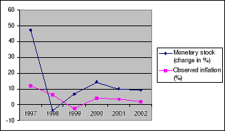
Table 3-2 shows the change in inflation and monetary stock. It can be seen that the change in M2 depends on how is the predominance in the change for NEA or NIA.

TABLE 3-2: MONETARY STOCK (M2), NET EXTERNAL ASSET (NEA) AND NET INTERIOR ASSET (NIA) IN PERCENTAGE

3.2.2 Exchange Rate Policy

The main objectives of Rwanda's exchange rate policy are to preserve the external value of the national currency and also to ensure the effective operation of the foreign exchange market. The instruments that are often used to conduct exchange rate policy are the rate of exchange and exchange regulations. The latter comprises all the arrangements resulting from the legislative texts and lawfully taken by the government in order to supervise the management of foreign currencies.

The flexible exchange rate regime was established in Rwanda in 1995 and at the same time the organisation and the management of the foreign exchange market were entrusted to the Central Bank.

The characteristic of the Rwanda flexible exchange rate regime is the fact that it is a controlled flexible policy. The mentioned policy pursues three main goals:

The instruments of the controlled flexible exchange regime in Rwanda are simply the rate of exchange reference and the interventions of the Central Bank on the foreign exchange market. The intervention of the Central Bank on the foreign exchange market conforms to the pattern of its mission of ensuring monetary stability and carrying out its objectives regarding the rate of exchange. This is done with the aim of correcting imbalances of liquidities of the market, as well as correcting the erratic movements of the national currency.

In other respects, there is a close link between the monetary policy and the exchange rate policy. Indeed, one of the principal counterparts of the money supply, which is the Net External Assets constitute an important source of monetary creation. According to this view, any positive balance of the balance of payments results in an increase in the money supply, while any deficit results in a reduction of the money supply. As a result, since the two policies aim either at the preservation of the internal value of the currency, or at its external value, their action must be harmonized for the stability of the currency.

With the help of international institutions such as the IMF and the World Bank, the Central Bank of Rwanda is trying to follow an objective, which entails developing a careful monetary policy, which will allow it to maintain harmony between the pace of the money creation and that of economic growth. The management of its stock change has contributed to reducing the exerted pression on the Rwanda currency and foreign payments. The harmony that has characterized the growth of the money supply and that of production has contributed to stabilize the inflation rate, the currency exchange offer has increased by 9% while it was 13.7% in 2000 (Republic of Rwanda, 2002: 10).

Through economic research, various models have been developed to better understand the monetary policy impact on the real economy and ultimately inflation. `The management of monetary policy consists to define the level of the instrument that, given the transmission mechanism of monetary policy, is consistent with the achievement of the target' (Martinez, Sanchez and Werner, 2000: 184). In the context of the conduct of monetary policy in several countries, the achievement of inflation target has become the fundamental goal of the monetary authority.

One way to evaluate the effectiveness of the monetary policy is by estimating the effect on the interest rate of the variables that should enter into the authorities reaction function. The Taylor rule mentioned previously is one of the more popular approaches to the empirical analysis of the reaction function. Indeed this rule works with the interest rate policy and the latter implies the open market operations, which are often taken as the most important monetary policy tool because they influence short-term interest rates and the volume of money and credit in the economy.

The monetary reaction function based on the Taylor rule has been used in both developed and underdeveloped countries. Judd and Rudebush (1998) quoted in Hsing, (2004) investigated and reviewed previous works and maintained that the Taylor rule is a valuable guide to characterize major relationships among variables in conducting monetary policy. Similarly, Romer (2001) quoted again in Hsing, (2004) analysed several issues in applying the Taylor rule. He noted that the values for the coefficients of the output gap and the inflation gap would change the effectiveness of monetary policy. Larger values of the coefficients would cause the actual inflation rate and output to decline more than expected. Due to a lag in information, it would be more appropriate to use the lagged values for the output gap and the inflation gap. The exchange rate and the lagged federal funds rate need to be included to incorporate the open economy and the partial adjustment process. Martinez, Sanchez and Werner (2000) analysed the mechanisms empirically by which the transmission of monetary policy has occurred in the Mexican economy from 1997 to 2000. Using VARS he found that the behavior of the real interest rate was determined by the traditional variables that guide the discretionary actions of any Central Bank and that this rate affected aggregate demand and credit in a statistically significant way. Applying the VAR model, Hsing (2004) estimated the monetary policy reaction function for the Bank of Canada. The results show that the overnight rate has a positive and significant response to a shock in the output gap, the inflation gap, the exchange rate or the lagged overnight rate. The author pursues the latter concluding that the main outcomes suggest that in pursuing monetary policy by the Bank of Canada, targeting output is as important as targeting inflation.

Sanchez-Fung (2000) estimated a simple Taylor-type monetary reaction function for Dominican Republic during the period 1970-98. He noted that the implicit reaction of such authorities suggest that they were more systematic during the period 1985-98 which might be attributed to a determination to» implicitly» follow feedback rules, rather than discretion, in monetary policy-making. Setlhare (2003) studying how monetary policy was conducted in Botswana by specifying and estimating an empirical monetary policy reaction for the Bank of Botswana over the period 1977-2000, identified a predominantly countercyclical policy reaction function. This reaction function suggests that inflation (directly and indirectly via the real exchange rate) is the ultimate variable of policy interest.

Smal and Jagger (2001) examined the monetary transmission mechanism in South Africa. The results of the model developed indicated that there was a fairly long time (one year) before a change in monetary policy affected the level of real economic activity, and another year before it had an effect on the domestic price level.

Sanchez-Fung (2000) however, observed that although the framework related to Taylor type monetary policy reaction has been implemented in the analysis of advanced economies, little work has been done for less developed countries.

The purpose of the following section will look at how monetary policy was conducted in Rwanda by specifying and estimating a monetary reaction function for National Bank of Rwanda.

4.1 EMPIRICAL ANALYSIS

4.1.1 Reaction function for Rwanda

Rwanda is a small open economy and it is necessary to examine how monetary policy reacts to output gap, inflation gap and exchange rate.

To formulate a monetary reaction function for National Bank of Rwanda the Taylor rule equation was adapted to the context of monetary policy in Rwanda. Indeed, Osterholm (2003) showed that the Taylor rule could be estimated where the rule has been used by Central Banks or at least be a close enough approximation to Central Bank behavior.

IG= the inflation gap which is (-^*), where is the actual inflation rate and ^* the target inflation rate.

The present study will follow suit by specifying and estimating a version of (1). That is, will be determined a variable that seems to be a plausible indicator of the stance of monetary policy in Rwanda. Evidence suggests that the short-term interest rate cannot be applied to the realities of developing countries when taken as an instrument in conducting monetary policy given the underdeveloped nature of the financial market. It has been argued that the monetary base is the most appropriate instrument to be used in developing countries (Sanchez-Fung, 2000).

Because of data availability problems for the monetary base series of Rwanda, the monetary stock aggregate (M1) will be used as the instrument policy. Indeed, the monetary stock aggregate (M1) plays an important role in Rwanda monetary policy since the National Bank of Rwanda assumed its responsibility to regulate liquidity in the economy and the data of the monetary base are frequently referred to M1.

In respect of goal variables, inflation and output will be used. The former variable has emerged from many economists as the real goal of monetary policy in order to maintain price stability and the latter is considered as a historically objective of monetary policy in various countries.

In the context of Rwanda, the strategy used by the Central Bank is to ensure that liquidity expansion is consistent with target inflation and GDP growth levels. Thus, the modified version of Taylor's rule to be estimated can be written as:

However, recently, with number of empirical studies related to the Taylor rule, economists argue that the exchange rate would also be an essential state variable that has to be included in the model in the case of a small and open economy (Osterholm, 2003). On this basis, the equation (2) is extended as follow:

ë₀, ë_1,ë_2,ë₃are constant term and coefficients respectively to be estimated empirically.

The equation (3) can be seen as a function in which the monetary stock aggregate (M1) reacts to the inflation gap, output gap and the change in exchange rate.

The version of the equation (3) to be empirically estimated can take a dynamic form since there is the lag response of Monetary Authority. On this basis, the equation (3) is expressed as follows:

M_t= ₀ + ₁M_t-1 + ₂IG_t + ₃IG_t-1 + ₄YG_t + ₅YG_t-1 + ₆DEX_t + ₇DEX_t-1 + _t (4)

Equation (4) is an autoregressive-distributed lag of order one [ADL (1, 1)]. This formulation allows one to consider that the forecast value of Mat time t is simply the reaction of monetary authorities to past and current economic states. Moreover, following Sanchez-Fung (2000: 9) one should consider that, statistically; equation (4) could help to justify the problem of wrongly measured data.

4.1.2 Methodology

4.1.2.1 Data

The econometric analysis of the version of Taylor rule retained for Rwanda will be undertaken using quarterly data during 1997 (Q1) - 2001(Q4), simply because the monetary authorities actually began to carry out monetary policy in an independent way from 1997. However, data for the variables after 2001(Q4) are not available.

Real GDP, Index of Consumer Prices, monetary stock aggregate and nominal exchange were obtained from the Central Bank of Rwanda and have been all transformed in logarithm form, except the Index of Consumer Price. In addition, the inflation rate is calculated as the change over four quarters of the seasonally adjusted harmonised Index of Consumer Prices and the inflation gap has been taken as the difference between the observed inflation and the inflation target. The Inflation target is not constant and was obtained from IMF and Rwanda (1995-2002) and the National Bank of Rwanda. Potential output is estimated based on the Hodrick-Prescott Filtering Process and the output gap is expressed as (Y-Y^*), where Y is the output and Y^* is the potential output. The monetary stock aggregate variable has been de-trended using the HP filter (see Pesaran and Pesaran, 1997). The nominal exchange rate reported is in terms of Rwandan Francs per US Dollar because of the extensive use of US Dollars to dominate international transactions (Republic of Rwanda, 2000: 369).

By using this data, the focus will be on estimating the model (4) using Microfit 4.0 and by checking whether the estimated parameters of the regression are meaningful to interpretation.

4.1.2.2 Time series properties of the data

Prior to carrying out the model, it is necessary to examine the time series properties of the variables included in it. This allows one to determine whether or not the regression is spurious. For this purpose stationarity of the data set is checked by using a simple appropriate test named Dickey- Fuller. The lag length used in the test is determined using the AKAIKE (AIC) and the Schwartz Bayesian Criterion (SBC) mainly. According to this criterion, the model to be preferred should have the highest AKAIK or the highest SBC.

Tables (4.1) and (4.2) present the integration test results for variables in their level form and in first difference respectively.

The results reported in Table (4.1) indicate that all the variables are stationary in levels except for the nominal exchange rate. The unit root for the variables, which are stationary, is rejected at all the conventional significance levels (the null hypothesis states that the time series has unit root and the alternative is that the time series does not have unit root).

From table (4.2) when the variables are transformed to their first differences, the ADF test rejects the null hypothesis about unit root at the all-conventional level of significance for all the variables except the inflation gap which rejects the unit root at the 5% level of significance. Therefore, all the variables are first - difference stationary. Overall, it can be concluded that all the variables in the model (equation 4), including the exchange, rate can be treated as I (0) because the exchange rate expressed in the model relates the change in the nominal exchange rate. Consequently, the Ordinary Least Squared (OLS) analysis by the feedback rule in which the monetary stock aggregate reacts to the inflation gap, the output gap and the exchange rate or all of them will provide non - spurious results.

Having the monetary stock aggregate (M1) as the dependent variable, one expects that the monetary stock aggregate will increase if inflation is below target, output is below the output gap, that is, the coefficient of YG and IG are expected to carry a negative sign. Regarding the change in the nominal exchange rate, we expect that the response of M to DEX would be negative.

4.2 Estimation results

Considering the full sample period 1997-2001, the coefficient of YG_t, YG_t-1 and DEX_t are insignificant and carry unexpected signs and the model fails the serial correlation and heteroscedasticity test. When reducing the model by taking out all the insignificant variables the final preferred model is specified as following:

This complies with most of the diagnostic statistics regarding no serial correlation, good functional form, normality and the absence of heteroscedasticity. On the other hand, the R² and the adjusted R² are fairly good and the signs of the estimated coefficient in the relation to their prior expectation are satisfactory.

The regression is significant as demonstrated by the F-statistic, which provides a test that the true value of the slope coefficients are simultaneously equal to zero (the p-value 0.003 is almost zero).

The goodness of fit, as measured by the coefficient of determination R², indicates how well the sample regression line fits the data. The fit indicates that about 64.4% of changes in monetary stock aggregate are explained by monetary stock aggregate in the one period lagged, the current inflation gap, the one period lagged inflation gap and the one period lagged change in the nominal exchange rate. When examining each explanatory variable it was found that:

- The response coefficients on inflation gap are about 0.96 and -0.65 respectively the contemporaneous and the one period lagged value.

- Both coefficients are statistically significant at the 5% level of significance.

- The response on the change in the one period lagged value of nominal exchange rate is(-2.45).

- Judging by the t-ratio, the coefficient is significantly different from zero at the all-conventional level of significance.

- The response coefficient on the one period lagged value of the monetary stock aggregate is about (-0.46) and judging by the t-ratio, the coefficient is significantly different from zero at the 10% level of significance.

(1) Considering the one period lagged value of the monetary stock aggregate (M_t-1), one can observe that a one percentage point change in the previous period monetary stock aggregate results in about 0.46% point change in the current monetary stock aggregate in the opposite sense, holding other things the same. This means that, there is one to 0.46 inverse relationship between the previous and the current monetary stock aggregate.

It is noticed that for a given change in the one period lagged deviation of the inflation from its target, the monetary stock aggregate reacts by a change of about 0.65 units. This impact seems statistically significant since the t-ratio is significant and the coefficient carries the right expected sign. This means that, if inflation were 1% point above its target, the Central Bank would decrease the monetary stock aggregate by 0.65% in terms of reaction, holding other things the same. Thus, the Central Bank was reacting to one period lag on the deviation of inflation from its target by a weight of about 0.65. Regarding the current period of inflation gap, the coefficient 0.96 can be interpreted as the change in the value of monetary stock aggregate following a unit change in inflation gap in the same period. That is, the monetary stock aggregate was changing in the same sense as the price level by 0.96% following a 1% change in prices.

The result shows that the Central Bank of Rwanda reacts to 1% change in the exchange rate by a change of 2.45% in the monetary stock aggregate inversely, holding other things the same.

In the light of the above findings, the Rwanda Central Bank's behavior in respect to the weight carried by the inflation gap in the current period and the one period lagged should be interpreted cautiously. Indeed, from the estimated of equation (4), the coefficient affecting the variable IG_t is positive and significant whereas the one affecting the variable IG_t-1 is negative and significant as well. This seems to show that the Central Bank reacts mainly to the inflation focusing on the one period lagged of the state of the economy while the positive contemporaneous relationship between the monetary stock and the inflation gap could be seen as the period of economic state adjustments. That is, dynamically speaking, in the current period the change in price leads the monetary policy to adjust the monetary base toward its trend. Overall, the change in the one period lagged in the exchange rate seems to be more influential than the inflation rate in explaining the change in monetary policy since the coefficient of the former carries the expected sign and its t-ratio is relatively very significant.

When looking at the result more closely with the objective of highlighting the variable that has influenced monetary policy decisions over the period of study, it is apparent that the monetary authorities were mainly concerned with the exchange rate. This is relevant given the importance of the exchange rate in a small, open, and developing country especially Rwanda, in the present case. Indeed, as noted previously, the exchange rate policy in Rwanda aims at approaching a balanced level of the exchange rate, to stabilise prices, to ensure a support for the growth and to connect Rwanda's foreign exchange market to the international market. These objectives are pursued under a controlled flexible policy regime, that is, the exchange rate can fluctuate from day to day but the Central Bank attempts to influence the exchange rate by buying and selling currencies in the foreign exchange market. The impact of such interventions is to affect the monetary base. According to this fact, the exchange rate considerations play a great role in the conduct of monetary policy and this has been shown through the estimation results. The exchange rate coefficient from the results leads one to consider that a depreciation of Rwanda Francs may lead the Central Bank to pursue a kind of contractionary monetary policy and similarly, an appreciation in Rwanda Francs may lead to pursue a high rate of money growth and such reaction consists basically in acquiring or selling of international reserve.

Given the fact that Rwanda has a strong dependence on assistance from multilateral financial institutions which in its turn has a real impact on the balance of payment, apparently, the importance of reacting to exchange rates seems to be relevant in Rwanda since it could limit the pressure exerted on the Rwanda currency in order to meet international prices and the debt service management. In addition, these findings about the exchange rate influence on monetary policy are consistent with the state of the Rwanda's economy from 1995 when it started to benefit from financial assistance from international institutions in the context of the Enhanced Structural Adjustment Facility (ESAF) and the Poverty Reduction and Growth Facility (PRGF). This may lead one to think that changes in the flow of international assistance could contribute to the significant changes in official reserves for the country. As a consequence, an objective of Rwanda currency stability should play an important role given the link between the foreign market operation and the change in monetary base and thereby the behavior of prices level. In this specific context, one could consider that monetary authorities were not as concerned about reacting to changes in the inflation as to the exchange rate simply because when focusing on the exchange rate, the Central Bank has also attempted to stabilize prices given the fact that the depreciation of Rwandan Francs and the increase in international prices affects the inflation rate.

Comparing these findings with the suggestion of the Taylor rule, it would appear that the weight of the inflation gap does not correspond to the Taylor rule's description which sets the weight greater than one. In addition, the estimates indicated a neglect of output gap as a goal variable under the period of study (see Table 4.3). These results may indicate that the Taylor rule adapted to the context of monetary policy in Rwanda expresses that the economy behaved by giving much importance to the exchange rate than to inflation and neglected the output change.

This dissertation intended to study how monetary policy was conducted in Rwanda. The task has been accomplished by designing and estimating a Taylor rule, monetary policy reaction function for the National Bank of Rwanda over the period 1997-2001.

Applying Ordinary Least Squared (OLS) on data taken from the National Bank of Rwanda, the Ministry of Economic and Finance of Rwanda and the IMF together, the study shows that the National Bank of Rwanda has had a monetary policy over the years with the monetary stock aggregates (M1) as the principal instrument.

- A contemporaneous inflation gap weight of (0.96), which is positively related to the monetary stock aggregate,

- A previous quarter inflation gap weight of (-0.65), which is negatively related to the monetary stock aggregate,

- A previous quarter change in exchange rate weight of (-2.45), which is negatively related to the monetary stock and

- A previous quarter monetary stock aggregate weight of (-0.46), which is also negatively related to the current monetary stock aggregate.

Judging these results according to the importance of each variable weight, one may be inclined to contend that while the National Bank of Rwanda reacted to the inflation from the previous quarter and the contemporaneous period, there was a much stronger response to the change in the previous quarter's exchange rate.

In general, such strong response of the National Bank of Rwanda to the exchange rate may reflect the economic environment in which the monetary policy was operating, because international aid has flow into Rwanda since 1995 in the context of various economic programs undertaken with the help of the International Monetary Found (IMF) or World Bank (WB). In addition, the estimate results indicated a neglect of output gap as a goal variable.

Given the fact that the Rwanda Central Bank claimed to be following the objective of preserving the internal and the external value of the currency in order to maintain harmony between the pace of the money creation and that of economic growth it may be suggested that the Central Bank of Rwanda should give more consideration to the way the output changes, that is, the Central Bank should respond to the variation of output gap following the influence of its change in the economic state.

In addition, the results of this study of course, are backward looking, in the sense that they represent the relationships that existed so far in the data. It is worth noting that a forward-looking model may enable the implantation of a more successful monetary policy rule for Rwanda and there may be areas for future research.

Blinder, A. S. (1999). Central Banking in theory and practice. Massachusetts: The MIT Press

Daniels, J. , Vanhoose, D. (1999). International monetary and financial economics. Cincinnati: South-Western College Publishing

Darnell, A. C. (1994). A dictionary of econometrics. Brookfield: Edward Edgar Publishing limited.

Dornbusch, R. , Fisher, S. , Startz, R. (2001). Macroeconomics. 8^th Edition. New-York: McGraw-Hill

Edwards, G. T. (1984). How economic growth and inflation happen. London: Macmillan Press

Enders, W. (1995). Applied econometrics time series. New-York: John Wiley and Sons.

Frowen, S. F. (1993). Monetary theory and monetary policy. London: The Macmillan press.

Meyer, L. H. (1980). Macroeconometrics, a model bulding approach. Cincinnati: South Weatern Publishing Co.

Mishkin, F. S. (1997). The economics of money, banking and financial. 5^th Edition. Massachusetts: Addison-Wesley

Pesaran, M. H., Pesaran, B. (1997). Microfit 4.0. Oxford: Oxford University Press.

Alexander, W. E., Thomas, J. T. , Balino, Enoch, C. (1995). An Adopting Indirect Instrument of Monetary Policy. IMF Occasional Paper No 126. Washington.

Clark, T., E. (1994). Nominal GDP Targeting Rules: can they stabilize economy? Federal Reserve Bank of Kansas City. Economic Review, Third Quarter 1994

Federal Reserve System and Monetary policy (1979). Congressional digest, Vol 58 issue 4: p101 2p (AN 10584253)

Gidlow, R. M. (1998). Instrument of monetary policy in South Africa. south Africa Reserve Bank, January 1998.

Government of Rwanda (2001). Third United Nations Conference on the Least Developed Countries. Brussels, 14-20 May 2001. Action Prgramme for the Development of Rwanda 2001-2010.

Hsing, Y. (2004). Estimating the monetary policy reaction function for Canada. A VAR model. Southeastern Louisiane University. Vol.3 No.1 Appril (2004)

Judd, J. P., Motley, B. (1993). Economic Review Federal Reserve Bank of SanFrancisco. 1993. Pages: 3-11.

Judd, J. P. , Rudebusch, D. (1998). Taylor Rule and the Fed: 1970-1997. FRBSF Economic Review 1998, No3

Martinez, L. , Sanchez, A. , Werner, A. (2000). Monetary policy and the transmission mechanism in Mexico. BIS paper No8. Paper presented at the seminar on stabilization and monetary policy organized by the Bank of Mexico, November 2000.

Mishkin, F. S., Posen, A. S., McDonough, W. (1997) Special Issue on Inflation Targeting. Economic Policy Review. Vol3, No3. Federal Reserve Bank of New-York, 1997.

Mishkin, F. S. (1995). Symposia on the monetary transmission mechanism. The journal of Economic Perspective. Vol.9 No 4 (1995): 3-10

Musinguzi, P. , Opondo, H. (1999). Bank of Uganda Staff Paper. Vol 1. No 1. 1999.

Musinguzi, P. , Obwona, M. B., Stryker, D. J. (2000). Monetary and exchange rate policy in Uganda. African Economic Policy Discussion Paper No23, April 2000.

Republic of Rwanda (2000). Rwanda Development Indicator. Ministry of Finance, Kigali.

Republic of Rwanda (2002). Rwanda Development Indicator. Ministry of Finace, Kigali

Sanchez-Fung, J. R. (2002). Estimating a monetary policy reaction function for the Dominican Republic. Discussion Paper No 02/01 Department of Economics. University of Kent, UK.

Small, M. M. ,de Jager S. The monetary transmission mechanism in South Africa. Occasional Paper No.16, September 2001, South African Reserve Bank.

Stryker, J. D. , Rajaratnam, B. , Cassim, F. (2000) The effect of fiscal, monetary, and exchange rate policy on the South African growth and employment. TIPS 2000 Annual Forum September 2000.

Svensson, L. E. O. Inflation Targeting as a Monetary Policy Rule. Journal of Monetary Economics 43 (june 1999), pp. 607-54.

Taylor, J. B. The monetary transmission mechanism: an empirical framework. The Journal of Economic Perspectives, Vol 9 No 4 (1995): 11-26.

Worrel, D. (2000). IMF Working Paper. Money and Fiscal Coordination in Small Open Economies. WP/00/56. International Monetary Fund.

Bernank, B. Mishkin, F. S , Milhov. What does the Bundesbank target? Europen Economic Review, 4 (june 1997). ( www.nber.org/papers/w5764.pdf). Accessed july 2004

Christensen, A. M. , Nielsen, H. B. (2003). Has US monetary policy followed the Taylor Rule? A cointegration analysis. 1988-2002. JEL classification: C32, E52.

Esanov, A. , Merkl, C. , de Souza, V. (2004). A preliminary evaluation of monetary policy rules for Russia. Duestembrooker Weg 120 24 105 Kiel. Kiel Working Paper No.1201. ( www.uni-kiel-de/ifw/pub/kap/2004/kap120.pdf). Accessed July 2004

Federal Reserve Bank of SanFrancisco (2004). US monetary policy: an introduction.

Hsing Y. (2003). Estimating the Bank of Japan's monetary policy reaction function. Working Paper.

IMF (2000). Policy for faster growth and poverty reduction in Sub-Sahara African and the role of the IMF. An IMF Issues Brief. ( www.imf.org) Accessed March 2004

IMF (2001) IMF concludes article IV consultation with Rwanda. Public information notice (PIN) No.01/31 March 27, 2001. ( www.imf.org) Accessed March 2004

IMF and Rwanda (1998-2001). Rwanda-enhanced structure adjustment facility economic and financial policy framework paper for 1998-2001. ( www.imf.org) accessed March 2004

IMF and Rwanda (1997-2001): Press release index for 1997-2001. ( www.imf.org) Accessed March 2004

Osterholm, P. (2003). The Taylor rule: a spurious regression? JEL classification: E52.

Sanchez-Fung, J. R (2000). Estimating a Taylor-type monetary policy reaction function for a small developing economy. JEL classification: E5

Setlhare, L. A. (2003) close look at Botswana's management of monetary policy: the reaction function approach.

Svensson, L. E. O. (1998). Inflation targeting as monetary policy rule. Working paper 6790 JEL No E42, E52.

Taylor, J. B. (1999). The monetary transmission mechanism and the evaluation of monetary policy rules. Third annual international conference of Central Bank of Chile on monetary policy rules and transmission mechanism. September 20-21, 1999 WP No.87

Taylor, J. B. (1998). An historical analysis of monetary policy rules. Working Paper 6768. Cambridge: National Bureau of Economic Research. ( www.nber.org/papers/w6768) Accessed April 2004

Walsh, C. E. (2001). The science(and art) of monetary policy. Federal Reserve Bank of Sanfrancisco. Economic Letter 2001-13, May 4, 2001.

Worrel, D. (2000). Monetary and fiscal coordination in small open economies. IMF working paper. WPI/00/56 JEL classification No.E63, E58

1995Q1-2004Q4	Real GDP	Consumption Price Index	Monetary stock aggregateM1
Quarter	In 10⁹ of Rwandan Francs	CPI	M1 in 10⁶ of Rwandan francs
1995 Trim I	71.37	306.98	29965.60
1995 Trim II	80.69	345.72	34220.00
1995 Trim III	88.74	395.55	39748.30
1995 Trim IV	95.62	400.87	40257.10
1996 Trim I	96.23	396.24	39886.70
1996 Trim II	102.62	397.09	42633.90
1996 Trim III	109.67	415.69	44305.80
1996 Trim IV	117.55	426.68	45831.00
1997 Trim I	130.81	433.68	48416.70
1997 Trim II	138.27	438.29	53079.60
1997 Trim III	144.51	454.87	52078.90
1997 Trim IV	149.70	492.21	56833.20
1998 Trim I	153.06	495.79	49267.20
1998 Trim II	156.19	496.86	53776.90
1998 Trim III	158.31	481.47	48530.40
1998 Trim IV	159.65	471.99	52877.50
1999 Trim I	156.05	474.42	51023.80
1999 Trim II	157.15	469.01	56578.70
1999 Trim III	158.78	475.05	57741.30
1999 Trim IV	161.19	480.57	58524.00
2000 Trim I	165.68	481.70	57119.80
2000 Trim II	168.79	485.65	57878.00
2000 Trim III	171.82	494.83	54857.20
2000 Trim IV	175.02	511.09	60281.50
2001 Trim I	177.77	514.17	57002.73
2001 Trim II	181.20	508.68	63415.20
2001 Trim III	184.67	507.33	61114.87
2001 Trim IV	188.48	508.76	65049.40

BIBLIOGRAPHY

Books
Backhouse, R. (1999). Applied UK macroeconomics.
Massachusetts: Basil Blackwell
Blinder, A. S. (1999). Central Banking in theory and
practice. Massachusetts: The MIT Press