2.1 Neural network vocabulary
In this paragraph, we explain the basic vocabulary needed to
understand Machine Learning algorithms or neural networks. All of this
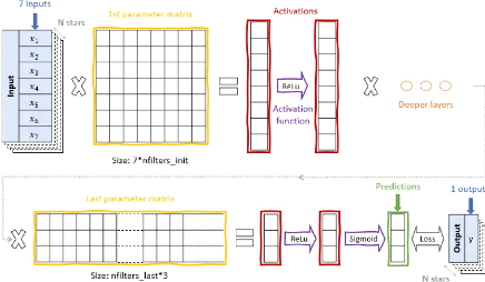
explanation will refer to Figure 2, which shows a visual example of a
neural net based on the data used for our first net, explained in Subsection
2.2.
As a first step, a neural network, also called a
net, can be considered as a black box algorithm, feeding on input data
in order to predict output data. Machine learning is almost always used for
images and computer vision but it also works on other data types like words,
time series or tabular data. The aim of a neural network is to train on a known
set of inputs and outputs to adjust itself, and finally to be used for
predicting unknown outputs based on known inputs. Physically, this technique
extrapolates the links between inputs and outputs within the black box and gets
to extend it to all inputs coming in a same way. For a net to work well, data
must be normalized between 0 and 1 (otherwise the huge number of matrix
multiplications can blow up values beyond the numerical precision range), and
well organized: there must be a training set, which contains inputs
and associated outputs and is used for adjusting the net predictions to those
outputs, and a test set, which is used to check the performance of the
adjusted net on a dataset it didn't train on. Furthermore, a net has to deal
with a huge amount of data but it cannot deal with everything at the same time:
it works on what is called a batch. The batch size is a hyperparameter
usually set to 64 (or another multiple of 2) but it is to be set by
taking into account other parameters. For this reason, it can be useful to
renormalize each batch before using it. This process is called
batch-normalization and is made by hidden layers called BatchNorm.
A net is structured in layers. The inputs are contained in the
input layer, the outputs in the output layer, both layers represented in blue
on Figure 2 and the black box is composed of layers referred to as
"hidden". Those hidden layers vary in number, size and complexity according to
the situation it is applied to. There are two types of hidden layers: the
parameters in yellow on Figure 2 and the activation
functions in purple on this same Figure. One can also speak about
activations (in red), the layers that don't require computing, which
help comprehension of what happens in the black box but is not used in the
process. The parameters can be considered as matrices that contain the
weights of the net, which are initially defined randomly or set to
arbitrary values and then adjusted in the training session. They can be for
example linear or convolutional layers. The activation functions are used to
help convergence during the training, and always keep the

Figure 2: Explanatory scheme of a neural
network for linear regression (see Equation 2.2.1). The net feeds on a N
× 8 dataset composed of 7 inputs (in our case photometric colours) in
the input layer and one output in the output layer. It has several hidden
layers (yellow and violet elements) whose number and type depends on the needs
of the situation, and obtains a prediction of the output. The activation
functions can be ReLu (maximum function), sigmoid or more complex if needed.
The loss function can be mean square error or otherwise, it helps compare the
predictions to the expected values and adjust the weights and bias (values of
parameters matrices) as needed.
dimensions of the activations they apply to. For example, the
ReLu layer is basically a maximum function helping the predictions to
stay positive (since data inside the hidden layers are supposed to be between 0
and 1), the sigmoid layer is often used as the last activation
function as it allows to project the predictions between 0 and 1, ensuring the
respect of normalization, or between expected minimum and maximum if one wants
to denormal-ize within the algorithm.
The adjusting part we have been talking about is what is
called training. It is a step during which the net feeds on the
training set inputs, which is called the forward pass, computes a
prediction and compares it to the expected outputs. This comparison can be done
using different techniques called loss functions. The type of loss
function is to be chosen in line with the situation for which one wants to
develop a neural network. For classification there is for example the cross
entropy loss function which turns the predictions into probability of belonging
to different categorical classes. For regression, one of the simplest examples
is root mean square error, but one can use more complex functions that are less
prone to bias from outliers. After obtaining the loss, i.e. the difference
between expectation and prediction using the loss function, the weights in the
hidden layers are adjusted so as to decrease this loss. This is called the
backward pass and is done by a method called an optimizer.
For all our nets, we will use the default setting which is the Adam
optimizer, a gradient descent technique using adaptive learning rate from
moment estimates. The learning rate is the rate at which the
adjustment goes, a very important
and useful hyperparameter which also has to be adjusted during
training. It is highly dependent on the batch size, so those two have to be
taken into account together. Once the backward pass is done, the whole process
starts over. One fitting loop is called an epoch, and the number of
epochs is another hyperparameter to choose and adjust carefully.
During one epoch, there is not only training but also a
validation part. This part consists of doing just a forward pass on the test
set, i.e. a set which is not used for training and so is unknown by the net, to
test its efficiency on real conditions. Thus, at the end of each epoch, one
gets two important pieces of information: the training loss and the
validation loss. One way to check if a net is learning is to get the
predictions and compare them visually with the expected outputs, thus showing
the evolution of the efficiency of the net during training. The training
process is supposed to tend to decrease the training loss

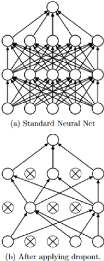
Figure 3: Illustration of dropout from
Srivastava et al. 2014 [1]. Up: a neural net with 2 hidden layers. Down: the
same net but thinned using dropout.
but sometimes it doesn't happen. This phenomenon is what is
called underfitting: the net doesn't catch the intrinsic links in the
training set and so can't improve itself. The validation loss doesn't take part
in the training process so it normally has no reason to decrease with the
number of epochs. If it does, everything is going well and the net is learning.
If it gets bigger, the net is overfitting: it becomes too specific to
its training dataset and is not able to extend to new data. One type of hidden
layer that can prevent the net from overfitting is Dropout. In fact,
overfitting can be seen as the net taking too much information from the
training dataset. So as to prevent from that, it is useful to skip some
parameters in the matrices as shown in Figure 3, an illustration of dropout by
Srivastava et al. 2014 [1], one of the first to develop this technique. The
upper net is fully connected, i.e. all of its parameters are active,
and in contrast, the second one has dropout. Dropout layers come with a dropout
probability, meaning a probability of dropping out a parameter in the following
layer. This quantity is another hyperparameter to optimize to improve the
performance of a net.
7
Therefore, creating a neural network requires one to organize
the data it will train on, decide of what type of net will be the most
efficient in this situation and adapt progressively all the hyperparameters to
get satisfying training and validation losses. Some of the hyperparameters will
of course depend on the situation, in particular as shown in Figure 2, the
sizes of the first and last parameter matrices depend respectively on the input
and output sizes. But basically, all other internal (number, types and other
sizes of hidden layers, loss function) and external (number of epochs, learning
rate) hyperparameters are to be adjusted by trial and error.
8
| 


