From pricing to rating structured credit products and vice-versa

From pricing to rating structured credit products and
vice-versa

Quentin Lintzer
Université Paris VI - Pierre & Marie Curie

Thesis submitted for the degree of:
Master M2 in Probability Theory and Applications

· September 2007 ·

Abstract

Credit risk area is one of the most rapidly developing areas in finance. A wide range of synthetic structured credit products builds on liquid credit instruments such as Credit Default Swaps, credit indices or Credit Synthetic Obligations (CSO) referenced on the latter. In this document, we first recall the principles of CSO pricing in a one factor gaussian copula model and outline two numerical procedures aimed at mapping joint loss distributions. We also formalize the theoretical modelling framework of Moody's, a rating agency, for rating Constant Proportion Debt Obligation (CPDO) and Constant Proportion Portfolio Insurance (CPPI) products. We then present our conclusions regarding an innovative Dynamic Proportion Portfolio Insurance (DPPI) product and raise some risk management issues.

Contents

1	Structured credit products: a business review 1.1 Introduction 1.2 Elementary building blocks			4 4 4
		1.2.1	Credit Default Swaps	4
		1.2.2	Credit indices	6
		1.2.3	Collateralized Synthetic Obligations	6
		1.2.4	Structured Non-Correlation Products	9
2	Modelling and pricing CSO tranches			12
	2.1	Modelling a CSO tranche payoff		12
	2.2	Default and premium legs of a CSO tranche		12
		2.2.1	Default leg	13
		2.2.2	Premium leg	13
		2.2.3	Fair premium	13
	2.3	The semi-analytic approach: one factor Gaussian Copula model . . .		14
		2.3.1	Copula functions: basic properties	14
		2.3.2	The one factor gaussian copula model	14
	2.4	Back to CSO tranche pricing: computing the expected portfolio loss		16
		2.4.1	Monte-Carlo simulations	16
		2.4.2	Evaluating the loss characteristic function	16
		2.4.3	Andersen's recursive formula	17

3 Modelling and Rating Dynamic Proportion Portfolio Insurance prod-

ucts 19

3.1	Moody's approach to rating CPDO and
	CPPI/DPPI products		19
	3.1.1	Historical vs risk-neutral probability measures	19
	3.1.2	Moody's Metric and coherent risk measures	20
3.2	Modelling risk factors		23
	3.2.1	Credit spread processes influenced by defaults and ratings . .	23
	3.2.2	Rating migrations and default events	24
	3.2.3	Interest rates process and other parametres	26
3.3	Portfolio investment rules		27
	3.3.1	Dynamic leverage function	27
	3.3.2	Deferred coupons	29
	3.3.3	Other key structural features	30
3.4	A study of the DPPI's sensitivities		30
	3.4.1	Tailor-made structural features to achieve target rating. . . .	31
	3.4.2	Hypothetical stress-scenarios	35

3.5 DPPI: any hidden pricing issue? 36

3.5.1 From the investor's perspective 36

3.5.2 From the investment bank's perspective 36

Conclusion 37

Appendix 38

Bibliography 42

List of Figures

1.1	Cash flows of a Credit Default Swap with physical delivery	5
1.2	Structuring of a single-tranch CSO	7
1.3	Structuring of a first-generation CPDO, referencing credit indices . .	9
3.1	Moody's rating conversion table	21
3.2	Moody's idealized EL values by rating category and tenor	22
3.3	DPPI base-case loss distribution conditional on the structure not cash-
	ingin	31
3.4	Distribution of cash-in times	31
3.5	Estimated expected loss as a function of S.	32
3.6	Estimated expected loss as a function of è (2000 simulations per
	coupon level)	33
3.7	Loss and Moody's Metric as a function of OL and TM, 1000 simula-
	tions per couple of parametres	34
8	Parametres of Moody's CDS spread processes	39
9	Correlation matrix of Moody's CDS spread processes	39
10	Moody's 10Y corporate rating transition matrix	39
11	DPPI optimized structural features	40
12	DPPI reference portfolio	41

Chapter 1

Structured credit products: a

business review

1.1 Introduction

Credit derivatives markets have been consistently among the fastest growing areas of capital markets in recent years: 2006 year-end ISDA survey shows outstanding notionnal of 34,000 USD Bio for all credit derivatives contracts, up from 8,000 USD Bio in 2004. Such a growth was fueled by the appetite of various types of investors for credit risk and relied upon the ability of investment banks to repackage credit risk into synthetic structured products.

Before going into the details of modeling and pricing such credit derivatives, we shall describe the principles of the main products that can then be used as building blocks for more sophisticated ones. They share the same underlying risk, that is the credit risk of one or several reference entities, whether it be a corporate company, a financial institution or even a soveriegn entity:

· Single-name Credit Default Swaps (CDS) are to credit derivatives markets what single-name equity stocks are to equity derivatives markets;

· Collateralized Synthetic Obligations (CSO) aim at tranching credit risk on an entire portfolio of reference entities, hence creating correlation risk;

· Constant Proportion Dynamic Portoflio Obligations (CPDO) and Constant Proportion Portfolio Insurance (CPPI) products allow investors to take credit risk on diversified portfolios of single names while avoiding first-order correlation risk;

· Vanilla options on credit indices started trading as liquidity in underlying CDS contracts and standardized CSO tranches was increasing.

1.2 Elementary building blocks

1.2.1 Credit Default Swaps

A Credit Default Swap (CDS) is a contract whereby counterpart A (the «protection
seller») receives a periodic premium from counterpart B (the «protection buyer») and
agrees to protect the latter against the default of entity C (the «reference entity»).

In the event of default, counterpart A would pay counterpart B the notional amount of a reference obligation (which could be a bond or a loan) issued by entity C and receive the reference obligation.

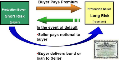
Figure 1.1: Cash flows of a Credit Default Swap with physical delivery

CDS are quoted in terms of spread (measured in basis points) over an Inter Bank Offered Rate (EURIBOR or LIBOR depending on the currency). Assuming a constant recovery rate R for the underlying obligation, we can easily express this spread as a function of the survival cumulative distribution function S0(.) of the reference entity defined as follows under the risk neutral probability measure Q. Let r be the continuous random variable modelling the instant of default:

?t ? R⁺,S0(t) = Q(r = t)

By construction, for a given notional amount N, a fixed recovery rate R, a contract maturity of T_n and risk-free bond prices B(0, Ti), i ? {1, .., n}, the market spread at inception of a given CDS is determined such that the present value of the premium leg (the «fixed leg») equals that of the default leg (the «variable» leg):

_Xn B(0, Ti) · E^Q [N(1 - R)1{Ti-1=ô=Ti} ~

i=1

_Xn B(0,Ti) · N(1 - R) · [S0(Ti-1) - S0(Ti)]

i=1

[ Xn ]

= EQ B(0, Ti)sN¹{ô=Ti}

i=1

_Xn B(0, Ti) · sN · (Ti - Ti-1) · S0(Ti)

i=1

As a result, the CDS spread s is given by the following formula, where D0(Ti) := B(0, Ti)S0(Ti) denotes the risky bond price:

s = (1 - R) ·	>n (S0(Ti_1) ) i=1 D(0, Ti) S0(Ti) - 1		(1.1)

1.2.2 Credit indices

Credit indices are convenient proxys for taking credit exposure on diversified portfolios of single names. They can be sorted by geographical criteria (Europe, Asia, US, Japan, Emerging markets), by industrial sector (e.g. Financials) or by debt riskiness criteria (investment grade, high yield). Among all indices, one shall bear in mind the ones detailed hereafter:

Index name	Debt riskiness		Characteristics	CDX.NA.IG
Investment grade	Diversified portfolio of 125 North American liquid corporate credits		CDX.NA.HY
High Yield	Broad-based portfolio of 100 high yield credits, i.e. sub-investment grade		ITRAXX IG
Investment grade	Diversified portfolio of 125 European liquid corporate credits		ITRAXX XOVER
High Yield	Diversified portfolio of 125 European high yield credits, i.e. sub-investment grade

Similarly to single-name CDS, they are quoted in terms of spread (measured in basis points) over LIBOR/EURIBOR rate. Given that all single-name components are equally weighted in credit indices, an event of default on a single name triggers a proportionate reduction in the notional amount of the index and a lump sum payment from the protection seller to the protection buyer.

1.2.3 Collateralized Synthetic Obligations Basic principles

Collateralized Synthetic Obligations (CSO) are securities issued by a Special Purpose Vehicle (SPV) and backed by a portfolio of credit protection-selling positions taken through several (usually over 100) CDS. The liabilities of the SPV get sliced into several CSO tranches that get hit sequentially in case one or more reference entities within the underlying CDS portfolio default. As a result, the fair premium of any tranche, usually expressed as a spread over 3-month LIBOR/EURIBOR rate, eventually depends on the joint-loss distribution of the underlying CDS portfolio.

CSO tranches can be defined by their attachment and detachment points:

· The attachment point l of the tranche is expressed as a percentage of the investment notional. It is the portfolio loss lower threshold above which the tranche's principal gets hit if one or several reference entities default within the portfolio.

· The detachment point u > l of the tranche is expressed as a percentage of the investment notional. It is the portfolio loss upper threshold above which the tranche's principal gets wiped out after one or several events of default.

CSO tranches are labelled upon their seniority in the capital structure:

· The equity tranche has the lowest attachment point of the structure - 0% - and usually a detachment point below 3%. Hence it is the riskiest tranche of the structure.

· The super senior tranche has the highest attachment point of the structure - usually around 22% - and a detachment point of 100%.

· Mezzanine tranches have an attachment point above the equity's detachment point and a detachment point below the senior's attachment point.

· Senior tranches have an attachment point above the mezzanine's detachment point and a detachment point below the supersenior's attachment point.

Unlike cash Collateralized Debt Obligations (CDO), CSOs are not backed by a portfolio of physical bonds or loans but by a portfolio of CDS contracts. This latter feature allows much more flexibility in structuring tailor-made securities than cash-based CDOs:

· Physical bonds or loans only exist in limited quantity, whereas CDS contracts
can be created as long as two counterparties agree to trade with each other;

· Whenever a cash-CDO is structured, all tranches must be sold to the investors, i.e. the deal must be fully syndicated, unless the CDO-arranging bank wants to keep some risk in it books, whereas CSO tranches can be structured independently because their payoffs can be replicated through model-based offsetting CDS positions.

· Transaction follow-up duties are heavier for cash-CDOs than for CSOs: for instance, loans can be subject to contingent early repayments.

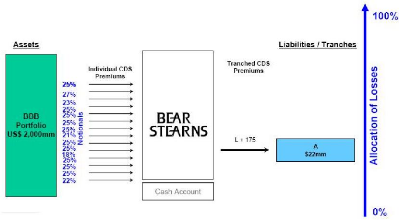
Figure 1.2: Structuring of a single-tranch CSO

CSO tranches on credit indices

As mentioned earlier, the price of a CSO tranche, which is defined by its attachment and detachment points within the capital structure, is a function of the joint-loss distribution of an underlying reference CDS portfolio. This joint-loss distribution function can be modeled in terms of two sets of parametres:

· single-name CDS spreads can be seen as proxies for valuing the default risk of each reference entity;

· cross-asset default risk dependency parametres, i.e. «correlation», that aim at describing the joint default-behaviour of a portfolio of reference entities.

The rationale for setting up a liquid market for tranches with standardized characteristics (attachment and detachment points) and referencing standard CDS portfolios (typically ITRAXX IG or CDX.NA.IG for 3,5,7 and 10 year-maturities) was to make correlation tradable, thereby allowing flexible correlation hedging for structured credit products.

Given that this market for standardized CSO tranches on credit indices aims at pricing correlation only and not default risk on any single name, tranches are quoted in terms of credit spread (measrued in basis points) on a Delta-Exchange basis: in other words, tranches and offsetting CDS positions are traded at the same time so that the resulting exposure of the investor is only to correlation and not to single-name first-order spread risk. Unlike other tranches which are quoted as a full running spread, the equity tranche (0%-3%), which is the riskiest slice of the capital structure, is quoted on a running basis assuming the protection seller on this tranche receives a 5% upfront premium.

Bespoke Collateralized Synthetic Obligations

Bespoke CSOs are tailor-made versions of CSO tranches on credit indices: the underlying CDS portfolio can be customized, as well as the characteristics of the tranche. This range of products offers more flexibility than standard tranches, for it allows the investor to choose his own credit risk profile by playing with the shape of the joint-loss distribution function (bespoke CDS portfolio) and choosing the attachment/detachment points that suit his aversion to risk.

In addition to tailoring the initial underlying CDS portfolio to the investor's needs, investment banks usually propose managed versions of bespoke CSOs that allow the underlying CDS portfolio to be revised later on in the transaction's life: the arranging bank appoints an external credit risk manager whose role is to manage actively the underlying CDS portfolio by making substitutions and weight adjustments among referenced single names.

Options on credit indices and tranches

As the liquidity of credit indices keeps improving, bid-offer spreads decrease and investment banks start proposing swaptions on major credit indices (ITRAXX XOVER, ITRAXX IG, CDX NA IG,...) on standard maturities (roll dates, i.e. 20-Mar, 20- Jun, 20-Sep, 20-Dec) and tenors (3Y,5Y,7Y).

1.2.4 Structured Non-Correlation Products

Unlike CSO tranches, the value of which relies heavily on correlation assumptions linking default probabilities on single names, a range of «correlation-free» structured credit products has emerged since 2004. Constant Proportion Portfolio Insurance (CPPI) and Constant Proportion Debt Obligation (CPDO) products reference CDS portfolios, but their joint-loss distribution is not tranched among investors.

Constant Proportion Debt Obligation: «the more you lose, the more you bet»

First introduced by ABN-Amro in S2 2006, a Constant Proportion Debt Obligation is a security whose principal and coupons are rated AAA by rating agencies such as S&P and Moody's and that pays to the noteholder quarterly EURIBOR/LIBOR coupons plus a spread around 100-200 bps depending on issuing market conditions. Such a return is achieved by selling credit protection on credit indices or on a portfolio of single-name CDS in an amount that is adjusted dynamically throughout the transaction's lifetime: this dynamic «leverage» function can reach as much as 15 times the initial notional.

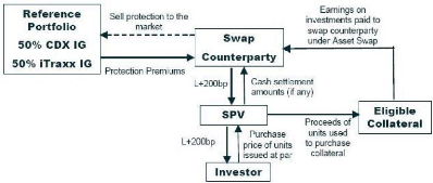
Figure 1.3: Structuring of a first-generation CPDO, referencing credit indices

Let us define the following variables at time t in order to summarize the few investment guidelines that rule the CPDO's behaviour:

· A = Notional of the security;

· NPV = Net Present Value of the security;

· MtM = Marked-to-Market value of all long positions on credit indices and/or single-name CDS;

· Collat = Value of the assets collateralized in the transaction to serve the EURIBOR/LIBOR component of the coupon;

· CA = Balance of the Cash Account of the structure; in particular, can be affected by default losses;

· TRV = Target Redemption Value of the security;

· PVNotional = Present Value of the security's Notional as discounted per the risk-free discount curve;

· PVCoupons = Present Value of the future coupons of the security discounted as per the risk-free discount curve;

· PVFees = Present Value of the future running fees to be paid by the noteholder and discounted as per the risk-free discount curve;

· TNE = Target Notional Exposure in credit indices or single-name CDS;

· F = Shortfall Multiplier, assumed to be constant in this example;

· lb = Lower Bound cash-out threshold, expressed as a percentage of the security's notional;

· TL = Target Leverage function.

The aim of the structure is to increase the security's NPV in order to hit the TRV (a «lock-in» event: in this case, the credit portfolio is unwound and the proceeds of the transaction are high enough to cover all future promised coupon, fee and principal payments until maturity by construction of the TRV aggregate. At the same time, the structure must avoid any «lock-out» event, which takes place when the security's NPV hits a fixed percentage lb, usually around 10%, of the security's notional N.

As long as no lock-in nor lock-out event has occured, the leveraging mechanism described hereafter expresses the Target Leverage function TL(t) as a linearly increasing function of the structure's shortfall, defined as the difference between the TRV and the NPV:

NPV (t) = MtM(t) + Collat(t) + CA(t) TRV (t) = PV Notional(t) + PV Coupons(t) + PV Fees(t) TNE(t) = F · (TRV (t) - NPV (t)) T NE(t) T L(t) = A

(1.2)

In other words, the CPDO's leveraging mechanism enables the structure to increase its credit exposure when the shortfall increases, i.e. when the security's NPV incurs MtM or default losses: «the more you lose, the more you bet». Conversely, MtM gains translate into a reduction in the structure's credit exposure.

Constant Proportion Portfolio Insurance: placing greedy but secured bets

Originally designed for equity underlyings, Constant Proportion Portfolio Insurance (CPPI) products referencing credit-linked assets have developped in the past three years. Unlike CPDOs, CPPIs are principal-protected at maturity. In other words, the investor will always receive the notional of the security at its maturity, whereas the CPDO noteholder can end up with as little as lb% of his initial investment.

The CPPI is a security whose principal is protected at maturity and whose coupons
can be rated by S&P and/or Moody's and/or Fitch. Similarly to CPDOs, the rated

CPPI pays to the noteholder quarterly EURIBOR/LIBOR coupons plus a spread around 50-100 bps depending on issuing market conditions. This return is achieved by selling protection on a portfolio of single-name CDS in an amount that is adjusted dynamically during the transaction's lifetime. This dynamic «leverage» function can reach as much as 10-12 times the initial notional.

Notations introduced earlier to describe the CPDO structure remain valid hereafter. In addition, we define the following variables at time t:

· BF = Bond Floor: value of a risk-free zero-coupon bond maturing at the legal maturity of the security;

· R = Reserve;

· RM = Reserve Multiplier.

A CPPI lock-out event happens whenever the security's NPV hits the Bond Floor BF. A lock-in event is the same as for CPDOs. The leveraging mechanism is different however: the CPPI's target leverage function TL is an increasing function of the Reserve R, defined as the difference between the security's NPV and BF.

R(t) = NPV (t) - BF(t) TNE(t) = RM · R(t) TNE(t) TL(t) = A

(1.3)

The CPPI's leveraging mechanism enables the structure to increase its credit exposure when the reserve increases, i.e. when either the security's NPV increases due to MtM gains or its BF rises as a result of lower interest rates. The more money you make, the more you can afford losing by increasing your bets.

Chapter 2

Modelling and pricing CSO

tranches

After choosing the pool of single-name CDS and defining the characteristics of the CSO tranche (attachment and detachment points), we want to determine a fair spread to be paid to the tranche buyer (i.e. the protection seller) as a fair reward for bearing this credit risk so that the present value of his investment is zero at inception (assuming no transaction costs nor fees to be paid to the arranging bank). Such a fair spread will eventually depend on the portfolio's joint loss distribution function accross time horizon L(t) until the CSO's maturity.

2.1 Modelling a CSO tranche payoff

Given an underlying portoflio of single name CDS, we assume that we have access to the joint loss distribution function L(t) of the portfolio at any time t, 0 t T, where T denotes the maturity of the transaction. We call respectively K and K the attachment and detachment points of our tranche. Its initial nominal amount is equal to K - K and the cumulative losses M(t) that affect that tranche at any time t is given by the following formula:

M(t) = (L(t) - K) - (L(t) - K)

We now assume that the underlying CDS portfolio is made of N reference obligors, each with a nominal amount A_n and a recovery rate R_n for n = 1,2, .., N. Let L_n = (1 - Rn)An be the loss given default of obligor n. Let r_n be the default time of obligor n. Let N_n(t) = ¹{ô_n=t} define the counting process which jumps from 0 to 1 when the n^th obligor defaults. The portfolio loss function L(t) is then given by:

L(t) = _XN L_nN_n(t) (2.1)

n=1

We note that the functions L(t) and therefore M(t) are pure jump processes.

2.2 Default and premium legs of a CSO tranche

Similarly to the approach presented for valuing the fair spread of a single-name CDS,
we determine the fair premium W * of the CSO tranche by equalizing the present

value of the default leg DL and the premium leg PL(W) of the tranche: by definition, W* solves the following equation:

PL(W^*) - DL = 0 (2.2)

The existence of a liquid market for standard CSO tranches based on ITRAXX and CDX indices provides us with a satisfactory framework for pricing credit default correlation among obligors, hence CSO tranches, under the risk-neutral probability. From now on, we assume that all expectations are taken under the risk-neutral probability measure.

2.2.1 Default leg

Given that M(t) is an increasing function, we can define Stieltjes-Lebesgue integrals with respect to M(t). The discounted payoff corresponding to potential default payments can therefore be written as:

I0

T n

_X ( )

B(0, t)dM(t) := B(0, ôj)Nj(T ) M(ôj) - M(ô- _j )

j=1

Using Stieltjes integration by parts formula and Fubini's theorem, the price of the default leg under the risk neutral probability measure can be expressed as:

I T J T

DL = E[ B(0, t)dM(t)] = B(0, T ) E[M(T )] + E[M(t)]dB(0, t)

0 0

2.2.2 Premium leg

Similarly, the price of the premium leg of the CSO tranche under the risk neutral probability measure is given by the folowing expression, where discrete premium payments are assumed to take place on _(Tj)j=1..m with T0 is the start date of the tranche and T_m = T is its legal maturity date.

? ?

m J Tj

P L(W ) = E ? B(0, Tj) W (K - K - M(t))dt_?

j=1 Tj-1

_Xm
j=1

J Tj

B(0, Tj)W (K - K)(Tj - _Tj-1) - E[M(t)]dt

Tj-1

2.2.3 Fair premium

We can now solve equation (2.2) for W * as a function of the expected cumulative tranche loss E[M(t)]:

B(0, T ) E[M(T )] + f 0 T E[M(t)]dB(0, t)

W * = (

>m ) (2.3)

(K - K)(Tj - _Tj-1) - f Tj

j=1 B(0, Tj) Tj-1 E[M(t)]dt

As soon as we can compute the expected tranche loss E[M(t)], the calculation of the tranche fair premium becomes straightforward. In order to do so, we then have to make further modelling assumptions on the behaviour of the joint tranche loss distribution M(t), or equivalently L(t).

2.3 The semi-analytic approach: one factor Gaussian Copula model

2.3.1 Copula functions: basic properties

Copula functions are useful tools for modelling dependency between random variables, for they allow to separate the univariate margins and the dependence structure from the multivariate distribution.

Theorem 1. Sklar's Theorem

Let F be a joint distribution function with margins F1, .., Fd. There exists a copula function C such that for all x1, .., xd in [-8, +8],

F(x1,..,xd) = C(F1(x1),..,Fd(xd))

Conversely, if C is a copula function and F1, .., Fd are the margins of respectively X1, .., Xd, then the multivariate function F of the vector (X1, ..Xd) is such that, for all x1, .., xd in [-8, +8],

F (x1, .., xd) = C(F1(x1), .., Fd(xd))

If the margins are continuous, then the copula function C is unique.

We shall need another key result in order to ensure copula functions are flexible enough to model joint loss distributions:

Proposition 1. Invariance

Let C denote the copula function of continuous random vector (X1, .., Xd). Let
f1, .., fd be strictly increasing functions defined respectively on the support of X1, .., Xd.
Then C is also the copula function of the continuous random vector (f(X1), .., f(Xd)).

We then recall the cumulative distribution function Ö of a standard gaussian variable and that of a multivariate standard centered gaussian vector with correlation matrix R:

x 1 Ö(x) = f8v2ð

e^-t2/^2dt

^x1xd11T 0-1y · dy1..dyd Ö_V xd) "

f8- f e2y

Definition 1. Gaussian Copula

Let (X1, .., Xd) be a gaussian vector with correlation matrix R, zero mean and unit variance. We can then express its copula function CR as follows:

CR(u1, .., ud) = Ö^`V^/) (Ö^-1(u1),..,Ö^-1(ud))

Given the invariance property of copula functions seen in proposition (1), CR is also the copula function of any gaussian vector with correlation matrix R.

2.3.2 The one factor gaussian copula model

Let (ô1, .., ôN) define the random vector of default times among the N obligors of
our reference portfolio. Given equation (2.1) and under deterministic assumptions
for recovery rates, determining the joint distribution of (ô1, .., ôN) is equivalent to

determining the joint loss distribution L(t) for all t = T.

We further assume that each default time random variable ôj, j = 1..N, follows an exponential law of parameter ëj. In other words, the cumulative distribution function Qj of ôj can be expressed as:

?t ? [0, T], P(ôj = t) := Q(t) = 1 - e_ëjt

We now wish to model the dependency between those default time random variables. The current market standard for doing so is to use the gaussian copula function CR where its correlation matrix R is defined as follows:

?

? ? ? ? ?

R=

?

?????

1 p ... p

p 1 ..

.. ..

... ...

. .. p

p ... p 1

Applying Sklar's reciprocal theorem, we can then exhibit the resulting cumulative distribution function Q of the random vector (ô1, .., ôN):

P(ô1 = t1,..,ôN = tN) := Q(t1,..,tN) = CR (Q1(t1),..,QN(tN))

A convenient way to simulate the random vector of default times (ô1, .., ôN) related together by a gaussian copula is to use an auxiliary random vector (X1, .., XN) modelled upon a single factor approach. We assume that all Xj, j = 1..N, depend respectively on a common standard gaussian factor Z and on an idiosyncratic standard gaussian factor Zj, where all Zj are mutually independent and independent from Z. Conditionnally on the common factor Z, all Xj, j = 1, .., N are therefore independent.

?j ? [1,..,N],Xj := vpZ + /1 - pZj

Proposition 2. The random vector (X1, .., XN) is a gaussian vector with correlation matrix equal to R.

Proof.

_v/

?

????????

=

...

0 vp

...

...

. ..

0

....

. .. ..

Z
Z1

...

·

?

???????

...
ZN

?

???????

?

????????

(X1, .., XN) = (vpZ + v/ 1 - pZ1, .., vpZ + 1 - pZN) vp -v1 - p 0 ... 0

...

....

. .. .. -v1 - p

0 vp

0 . . .

We have expressed (X1, .., XN) as an affine transformation of the gaussian vector (Z, Z1, .., ZN). Hence, (X1, .., XN) is a gaussian vector itself. The general term of its correlation matrix (pij,1 = i, j = N), is given by:

Cov (vpZ + v1 - pZi,vpZ + v1 - pZj) pij = V ar(Xi)V ar(Xj)

= äij(1 - p) + p

Hence, the correlation matrix of (X1, .., XN) is also R.

Applying invariance proposition (1) to the random vector of default times (ô1,.., ôN) Law = (Q^-1

1 (Ö(X1)), .., Q-1

N (Ö(XN)), we conclude that both vectors share the same gaussian copula function.

2.4 Back to CSO tranche pricing: computing the expected portfolio loss

We shall now present three numerical methods in order to evaluate the expected tranche loss function E[M(t)], Vt E [0, T]. We stress the fact that the following methods apply within the framework of the one factor gaussian copula model to a finite heterogeneous portfolio (i.e. in terms of individual nominal weights and recovery rates) of obligors with deterministic recovery rates. We shall not detail the well known analytic results that can be derived from Large Homogeneous Portfolios (LHP).

2.4.1 Monte-Carlo simulations

The Monte-Carlo approach is probably the most straightforward method to price a CSO tranche fair premium:

1. Simulate N +1 independent standard gaussian variables (Z, Z1, ..ZN) by using, for instance, the Box-Müller transform, the polar method or even by drawing in the random variable Ö^-1(U), where U is a uniform random variable; within the one factor gaussian copula model, the random vector (X1, .., XN) = ( /ñZ + /1 - ñZ1, .., /ñZ + /1 - ñZN) is therefore a gaussian vector with correlation matrix R.

2. Simulate (ô1, .., ôN) by drawing in the random vector

(Q^-1

1 (Ö(X1)), .., Q-1

N (Ö(XN))

3. Evaluate the tranche loss function M(t), Vt E [0, T] along this loss scenario;

4. Repeat steps 1 & 2 and evaluate the tranche loss function along this new loss scenario;

5. Loop on step 4 until you feel comfortable (confidence interval or variance criteria) with the convergence of the empirical estimate of E(M(t)), Vt E [0, T];

6. Evaluate the CSO tranche fair premium detailed in equation (2.3). Such a simple anf flexible method comes at a high computation cost though, because one has to draw millions of random variables in the case of a reasonably large portfolio (between 100 and 200 obligors).

2.4.2 Evaluating the loss characteristic function

We first determine the expression of pj(t|Z), the cumulative distribution function of default time ôj, j = 1..N conditional on the common factor Z.

?j ? {1, .., N}, ?t ? [0, T], pj(t|Z) : = P(ôj = t|Z)

= P (Q6 ¹(Ö(Xj)) t|Z)

~ = PQ^-1(Ö(vñZ + ñZj)) = t|Z)

= P (Zj G ₄Ö^-1 (Qj(t)) v ñZ |Z)

(Ö^-1(Qj(t)) ? ?ñZ

v1 ? ñ )

- ñ

= Ö

We then derive the total loss characteristic function conditional on the common factor Z:

?u ? R, ÖL(t)(u|V ) : = E [exp(iuL(t))|Z]

= E [exp(iu EL_nN_n(t))|Z1

n=1

=

E [fl exp(iuL_nN_n(t)) | Z1

n=1

_YN E [exp(iuL_nN_n(t))|Z]

n=1

_YN [1 + p_n(t|Z)(exp(iuL_n) - 1)]

n=1

where we have used that (N1(t),..,NN(t)) are mutually independent conditionally

on the common factor Z.

We now integrate the conditional characteristic function over the common gaussian factor Z to retrieve the unconditional characteristic function ÖL(t):

+8

= IÖL(t)(u|z)dÖ(z)

?u ? R, ÖL(t)(u) : = E [ÖL(t)(u|Z)]

Once we have found the loss characteristic function, we can use the Fast Fourier Transform (FFT) to recover the loss distribution function itself, which we then plug into equation (2.3) to derive the CSO tranche fair premium.

2.4.3 Andersen's recursive formula

The recursive approach described in [1] builds on the fact that the portfolio loss function can only take a limited number of values. This set of values depends in turn on the obligors' individual loss given default levels L_n, ?n ? {1, .., N}. We now assume that all those loss levels can be expressed as multiples of a loss unit l:

?n ? {1, .., N}, ?a_n ? N, L_n = a_nl

?i ? {0,1, ..,

XN k=1

ák}, P (L = il) = i+8 Pz--z(L^(N) = L il)dö(z)

We further assume that all N obligors are ranked. The possible values for the loss function L are restricted to the following subset:

{m

L ? E _ájkl, m ? {1,..,N}, {j1,..,j_m} ? {1,.., N} ? {0} k=1

The power of Andersen's recursive algorithm is that it allows to compute the loss distribution while assuming that the pool of obligors results from the sequential addition of all obligors upon one specific ranking order. Let j ? {1, .., N} refer to the first j obligors added to the pool and L⁽j⁾ the discretized loss function associated

with that sub-pool. We can then express the loss distribution of L⁽j⁾ as a function of L(j-1).

Proposition 3. Andersen's recursive formula

Let j ? {1, .., N} and L⁽⁰⁾ = 0. Assume the loss distribution function L(j-1) conditional on the common factor Z is known. Let QZ denote the risk neutral probability measure conditional on the factor Z and pj the default probability of j^th obligor conditional on factor Z. Then we have the following recursive result:

?i ? {0, 1, .., _XN ák},

k=1

QZ (-⁰⁾ = il) = (1 - pj)QZ(L^(j-1) = il) + pjQZ(L^(j-1) = (i - áj)l)

Proof. Let Dj,j?{1,..N} denote the default indicator variable of j^th obligor conditional on the factor Z. Using the conditional independence of Dj,j?{1,..N}, we can then write for all j ? {1, ..,N} and for all i ? {0, .., Ejk=1 ák}:

QZ(L⁽j⁾ = il) = QZ(L⁽j^-1) = (i - áj)l,Dj = ¹) + QZ(Lj-1 = il, Dj = 0)

= QZ(L⁽j^-1) = (i - áj)l)QZ(Dj = 1) + QZ(L⁽j^-1) = il)QZ(Dj = 0)

= pjQZ(L(j-1) = (i - áj)l) + (1 - pj)QZ(L(j-1) = il)

Andersen's recursive formula evaluated at rank N thus provides the conditional loss distribution L^(N). The last step in the computation of the unconditional discretized loss distribution L is to integrate the conditional loss distribtion against the density function of the factor's standard gaussian law:

Chapter 3

Modelling and Rating Dynamic

Proportion Portfolio Insurance

products

Summer 2007's turmoil in global credit markets resulted in a significant increase in volatility, thereby threatening the rating stability of many existing structured products including CSO tranches and CPDOs. A straightforward response to such a volatile environment is to cap the downside Mark-to-Market risk by adding a capital protection feature to new structured products: Constant Porportion Portfolio Insurance (CPPI) products and their most recent offshoots, Dynamic Proportion Indurance Products (DPPI), belong to that category.

We shall first recall the main principles of Moody's approach for measuring risks in order to rate CPDO and CPPI/DPPI products and outline its main assumptions in modelling risk factors. We shall then describe the DPPI's major risk sensitivities and present some of its key structuring features in order to mitigate those risks. Finally, we shall analyze the DPPI's behaviour under several stress-scenarios.

3.1 Moody's approach to rating CPDO and CPPI/DPPI products

3.1.1 Historical vs risk-neutral probability measures

Before going into the details of rating and pricing DPPI products, we shall address the following question: why do investment banks price their structured products under a risk neutral probability measure while rating agencies rate them under the historical probability measure?

Rating agencies evaluate loss ditributions under the historical probability measure because investors are mainly concerned with knowing how likely it is that they are going to lose money in our real «historical» world. They don't care about such a likelihood in a risk-neutral world. Doing so requires rating agencies to estimate future historical default probabilities and loss distributions, the parametres of which are calibrated statistically, whenever it is possible, on past historical data.

On the other hand, investment banks are concerned with pricing such products by evaluating the associated hedging costs. Fundamental results such as HarrissonPliska's no-arbitrage pricing theorem and Black-Scholes conclusions ensure that:

· in a viable and complete market, there exists only one probability measure Q called «risk-neutral» under which discounted asset prices are martingales;

· there exists a self-financing portfolio that replicates the product's payoff.

Girsanov's theorem allows us to relate historical and risk neutral probability measures through the notion of risk premium, which in turn can be interpreted in terms of risk aversion: under most market circumstances, real-world investors are naturally risk-averse and hence require to be paid an extra return for bearing default risk as compared to its true historical insurance cost. Hence coexisting historical and risk-neutral probability measures serve different purposes: the historical approach prevails for weighting future real-world scenarios and building risk measures such as the Value-at-Risk, while the risk-neutral framework allows the pricing and the hedging of traded securities.

3.1.2 Moody's Metric and coherent risk measures

We now temporarily put the risk-neutral measure aside and focus on the historical probability measure. Moody's uses the same methodology to rate CPDO and CPPI/DPPI products. It estimates the expected present value of the loss function L(M) through Monte-Carlo simulations under the historical probability measure.

Definition 2. Moody's expected discounted loss

Let t E I = {0, ät, .., kät, .., T} describe the discrete time scale with T the maturity of the deal. Let Xt := (X⁽¹⁾

t , .., X(p)

t ) be the p-vector of risk factors observed as of date t. We introduce the filtration _(Ft){t?I} defined as ?t E I, Ft := ó (X_u,u E I,u = s). We further define the three stopping times (r, r, r):

r := inf{s = 0, NPV (s) = TRV (s)}

r := inf{s = 0, NPV (s) = BF(s)} A T r := r A r

We then express Moody's risky discount factor DF^(M) as a function of the EURIBOR/LIBOR rate curve and of the senior spread s served to the investor:

?t E I, DF^(M)(t) :=	t-1Y i=0	1
		1 + ät(EUR(iät, (i + 1)ät) + s)
>1p i=1 L(M) L(M) = i p			+	ót99%
				vp

Then, under the historical probability measure, Moody's expected discounted loss L(M) is given below:

[ ]

L(M) := E _1{ô<ô} [A(1 - sl) - max(NP V (r), BF (r)) + DI(r)]⁺ DF ^(M)(r)

where sl is the detachment point in % of the subordinated note.

In practise, Moody's uses an unbiased empirical estimator of L(M), ^L(M) defined as:

where t99% := Ö^-1(99%), p is the number of Monte-Carlo simulations, L(M)

i is the

loss calculatd on the i^th scenario and ó is the standard error of (L^(M)

1 , .., L(M)

p ).

Moody's then maps that value L(M) and the maturity of the deal T against a positive real scale S = [0, 21] through a function MM called «Moody's Metric»:

MM : [0, 1] × R⁺ -? [0, 21]

(x,t) i-? MM(x,t)

We shall now describe how the Moody's Metric mapping function works. We first define the letter-to-integer mapping function R:

R : {Aaa,Aa1,..,Ca,C} -? {1,..,21}

m -? R(m)

The discrete mapping table is given below:

Rating-Figure	Rating-Letter
1	Aaa
2	Aa1
3	Aa2
4	Aa3
5	A1
6	A2
7	A3
8	Baa1
9	Baa2
10	Baa3
11	Ba1
12	Ba2
13	Ba3
14	B1
15	B2
16	B3
17	Caa1
18	Caa2
19	Caa3
20	Ca
21	C

Figure 3.1: Moody's rating conversion table

We shall now define the discrete function EL that maps the integer equivalent of a rating category and a maturity with a percentage expected loss:

EL : {1, .., 21} × {1, .., T} -? [0, 1]

(m, t) '-? EL(m, t)

Moody's calibrates the function EL on historical default data by using the cohort method.

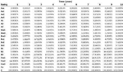
Figure 3.2: Moody's idealized EL values by rating category and tenor

We shall then define EL, the time-continuous version of EL function obtained by linearly interpolating EL between two discrete integer dates:

EL : {1,..,21} x [0,T] -*[0,1]

(m, t) i-* (t + 1 - [t])EL(m, [t]) + (t - [t])EL(m, [t] + 1)

Let us now define the reverse mapping function F ^-1 that transforms any percentage loss level and tenor into a rating:

F -1 : [0, 1] x [0, T] -* {1, .., 21}

(x,t) -* min{m E {1,..,21}| EL(m,t) = x}

We finally give the expression of the Moody's Metric function MM: Definition 3. Moody's Metric

?x E [0,1],?t E [0,T],

EL(F ^-1(x, t), t))

ln x - ln (

MM(x, t) := F ^-1(x, t) + ln ( EL(F ^-1(x, t) + 1, t)) - ln ( EL(F^-1(x, t), t))

In other words, the Moody's Metric can be seen as a standardized continuous scale that allows to compare expected loss levels for different tenors. We shall now take a closer look at the notion of risk measure and understand to what extent it makes sense to use the expected loss as a proxy for measuring risk.

Definition 4. Coherent Risk Measure

Let C denote a set of random variables representing all possible risky positions and L E C be a random variable whose range of values represents possible losses from any given risky position. We define the risk measure function p as a mapping from C to R. The risk measure p is coherent if it is:

i) monotonous: ?X, Y ? G, X = Y p(X) = p(Y )

ii) positively homogeneous: ?X ? G, ?h > 0, hX ? G and p(hX) = hp(X)

iii) sub-additive: ?X, Y ? G, X + Y ? G and p(X + Y ) = p(X) + p(Y )

iv) translation invariant: ?X ? G, ?a ? R s.t. X + a ? G, p(X + a) = p(X) + a

Proposition 4.

If G⁺ is a set of non-negative random variables, interpreted as a loss from a risky position, then expected value is a coherent risk measure:

?X ? G⁺, p(X) := E[X]

Proof. Properties (i),(ii), (iii) and (iv) immediately result from the expectation's linearity.

Unlike E[X], the Moody's Metric MM(X, t), where X is a positive random variable that takes its values in [0, 1], is not a coherent risk measure: though it is clearly monotonous and subadditive (because MM(., t) is increasing and concave), it is neither positively homogeneous, nor translation invariant.

3.2 Modelling risk factors

Moody's Monte-Carlo approach requires risk factors to be modelled and simulated. The complexity of the task for rating DPPI products comes from the fact that risk factors are numerous and can depend on each other. We assume that the DPPI's portfolio is initially composed of long CDS positions on N obligors. The 5Y CDS mid-spread and the rating of each obligor n, n ? {1, .., N}, are known at the deal's inception and are equal to (s_n(0),R_n(0)).

3.2.1 Credit spread processes influenced by defaults and ratings

Moody's assumes that individual 5Y CDS spread processes follow a generalized Vasicek diffusion process specific to rating groups. The 21 available rating categories are grouped into 8 rating groups {Aaa, Aa, A, Baa, Ba, B, Caa, Ca/C}. Let j ? {1, .., 8} denote the rating group's index. Then (S(t) = (S1(t), .., S8(t)))t?[0,T] is the associated 8-dimensional spread random process. We then give the stochastic differential

equation ruling the spread process (S(t)), where (á, â, ã = 1, ó, ó, ADR, ADR, a, b, p)
are historically calibrated parametres of the diffusion process and t0 is equal to 1 year:

?j ? {1, .., 8}, ?t ? [0, T], dSj(t) = á(â - Sj(t))dt + min(ó, óS^ã_j (t))dW (j)

t

where

? ????? ?????

â = â min (ADR,max (ADR, aADR(t) + b)) if t = t0 PN n=1 Ln(Nn(t)--Nn(t--t0)) ADR(t) = PN if t = t0 n=1 An â = â if t < t0 ?(i,j) ? {1, .., 8}^2, d (W(i), W(j)) t = pijdt

(3.1)

and Sj(0) = Sj,0

Equation (3.1) is remarkable for several reasons. First, given that ã = 1 and that the
spread process is continuous, it doesn't allow credit spreads to be negative. Second,
it models a dependency between the spread process itself and default events through

the parametres (ADR, ADR) and the variable ADR(t): the idea is to make the current long term mean 3 depend on the portfolio's Average Default Rate ADR(t) such that 3 is stressed for a limited time period equal to t0 after any event of default and tightens in default-free environments. Third, it accounts for a dependency between the obligor's rating and its spread process: whenever an obligor's rating group changes, its associated spread process is updated accordingly. Fourth, the random noise source (Wt = (W1(t), .., W8(t))) is a correlated 8-dimensional brownian motion.

Such dependency relationships are far from being flawless though: one could argue that they do not account for default events occuring outside the portfolio's pool of obligors. One could also demonstrate that individual spread processes are not driven by their belonging to a rating group, but more by marketwide, firm or industry specific events that are not necessarily reflected in a rating change.

In order to simulate a CDS spread for any tenor, Moody's assumes that the term structure of spreads is deterministic, calibrated on historical data and specific to each one of the 8 rating groups defined above. Though such an assumption may seem highly questionable at first and lead to obvious arbitrage opportunities, Moody's solves the issue by requiring stress scenarios to be run with a flat term structure while preserving a stressed Moody's Metric level.

3.2.2 Rating migrations and default events

Moody's simulates rating migrations and default events within a multi-factor gaussian copula framework applied to a markovian multi-period rating transition model. The first input of this model is a square rating transition matrix over a given time horizon T, noted MT E M_p(R), where p denotes the number of potential rating categories of the obligors, including one default category. Moody's assumes there are 18 of them, the mapping of which can be derived from figure (3.1) with categories Caa - C merged and an extra default category D with rating 18.

The rating path of the n^th obligor, j E {1, .., N}, until time horizon T is given by the random process (Rn(t))t?[0,T]:

R_n : Ù × [0,T] -? {1,..,18} (ù,t) -? R_n(t)(w)

We then recall the definitions of a generator matrix and of a time-homogeneous Markov process

Definition 5. Generator Matrix

Assuming A E M_p(R) with general term _{(ëij)(i,j)?{1,..,p}2.} Then A is called a generator matrix if:

i) Vi E {1, ..,p}, >ip j=1 ëij = 0

ii) V(i,j) E {1,..,p}², i =6 j ëij = 0

Definition 6. Time-homogeneous Markov process

X is a time-homogeneous Markov process with generator Ë if:

?t = 0, ?Ät > 0, ?(i, j) ? {1, .., p}², P(X(t + Ät) = j | X(t) = i) = (e^ËÄt)_ij

We now assume that _{(Rn(t))tE[0,T]} is a Markov time-homogeneous process with generator matrix Ë. We introduce the transition matrix MÄt over time period Ät through its general term (pij)(i,j)<p:

?t ? [0, T, ]?(i, j) ? {1, .., p}², pij := P (R_n(t + Ät) = j | R_n(t) = i)

It is worth noting that pij does not depend on t because of the time-homogeneous property of _{(Rn(t))tE[0,T].} As a direct consequence of R_n's definition, we have the following property:

Proposition 5. Composition of transition matrices Assume Ät is such that TÄt ? N^*. Then:

T } k = M_T^TÄt

?k ? {1, ..

Ät

We shall now describe briefly Moody's multi-factor gaussian copula model: similarly to the one factor gaussian copula model, the idea is to draw a random vector X = (X1, .., XN) from a gaussian law with a given correlation matrix Ó, where the latter depends on several factors. Let us define (Z^G, Z^I, Z^I,R) as three independent standard gaussian factors that account for respectively the global state of the economy, the state of any specific industrial sector and for a combination of both industrial and regional factors. For any given obligor n ? {1, .., N}, let us define e_n as an idiosyncratic factor that follows a standard gaussian law and that is independent from the common factors (Z^G, Z^I, Z^I,R) and from all other idiosyncratic factors. Then, for all n ? {1, .., N}, one can affect the state variable X_n to n^th obligor:

qXn _ñG ZG ñ^I_nZ^I VñIn ,R _ZI,R \ + 1 - ñG -ñ^I_n -ñn I,Ren

The random vector X is a gaussian vector with zero mean and a correlation matrix Ó given below. The correlation parametres (ñ^G_n , ñ^I_n, ñn ^I,R) are specific to each obligor and depend on some characteristics of their businesses in terms of industry and operations' scale. They are picked up from a subset of values subject to Ó remaining positive definite.

?

? ? ? ? ?

Ó=

?

? ? ? ? ?

1 ñ12 . . . ñ1p

.

.

ñ21 1 .

. .

.

...

...

. ..ñp-1,p

ñp1 . . . ñp,p-1 1

with:

q? (i, i) ? { 1, .., p}² ñij ñG Vñi ,Rñj,R

Applying well known results on the generalized invert of the distribution function of (R_n(t + Ät)|R_n(t)), we can write the following proposition:

Proposition 6. Rating transition simulation

Let us assume that each obligor's rating is likely to be confirmed or revised only on

the following dates {Ät,..,kÄt,..,mÄt}, where m := T/Ät ? N^*. Let F -1

k,Ät, k ?

{1, ..,p} denote the generalized invert of the cumulative distribution function of rating transitions over time period Ät starting from initial rating category k. We recall that Ö is the cumulative distribution function of the standard gaussian law and that (X1,..,XN) is the gaussian vector with correlation matrix Ó describing the state of our N obligors. We finally assume that initial ratings (R1(0),..,RN(0)) are known. Then the rating of each obligor on discrete dates {Ät,..,kÄt,..,mÄt} can be expressed through the recursive formula:

?k ? {1, .., m}, ?n ? {1, .., N}, R_n(kÄt) = ^FR,¹_:((k-1) Ät),Ät (Ö(X_n))

Moody's uses its historical database of rating transitions and defaults over time horizon T to build the marginal cumulative distribution functions (Fk,T)k?{1,..,p} and MT through some cohort method. Assuming _{(Rn(t))t?[0,T]} is a Markov time-homogeneous process, one can infer MÄt thanks to proposition (5) and use proposition (6) to simulate N correlated rating paths. The rescaling of matrix MT comes at a cost however: given the choice of the gaussian copula, one can show that when Ät --? 0, joint default times (ô(Ät)

1 , ..,ô(Ät) ^N) become independent: a way to address this issue is to stress Ó as Ät gets smaller so that the correlation structure is somehow preserved. In the case of the DPPI, T is equal to 10 years and Ät to 6 months.

3.2.3 Interest rates process and other parametres Interest rates

Moody's interest rate model is based on projecting a daily evolution of 3-month and 10-year term rates and linearly interpolating between them for rates of other tenors. Rates with tenors shorter than 3 months are assumed to be equal to the 3-month rate. 3-month and 10-year term rates follow a two-dimensional correlated Cox-Ingersoll-Ross (CIR) process, where R^s and R^l denote respectively 3-month and 10-year term rate processes:

?

??? ?

????

dR^s_t = ás(âs -- R^s_t)dt + ópR^s tdW s dR^l_t = ál(âl -- R^l_t)dt+ó JR^l_tdW_t^l

d (W^s,W^l)_t = ñdt

(Rs0, R^l ₀) = (r_s, rl)

In order to make sure that Euler's discretized sheme does not generate negative values for interest rates, the natural discretized CIR process is given below:

(R^s₀, Rl0) = (r_s, rl)
?k ? {1,..,T/Ät},

?

?? ?

???

(3.2)

R^s(kÄt) = |R^s((k -- 1)Ät) + ás(âs -- R^s((k -- 1)Ät))Ät + .. + ÄtR^s((k -- 1)Ät)Z1|

R^l(kÄt) = |R^l((k -- 1)Ät) + ál(âl -- R^l((k -- 1)Ät))Ät + .. + ó₀/ÄtR^l ((k -- 1)Ät)(ñZ1 + ñ²Z2)|

Recovery Rates

Default recovery rates for our N obligors are assumed to be random and follow marginal Beta distributions correlated through a one factor gaussian copula model. Given that the recovery rate RR_n of each obligor n follows a Beta distribution, it is characterized by its mean li_n and standard deviation ó_n. li_n and ó_n depend on the obligor's location, its type (corporate, sovereign,..) and the seniority of the CDS underlying reference obligation. The parameters á_n and O_n of the Beta(á_n, O_n) distribution are given below:

2 1-u

?n ? {1, .., N}, { á_n = li_n ó2 ¹⁴¹1^-un 1 \

)

O_n = (1 -- lin)(lin ón 2 1

Let RRG Law = N(0,1) denote the global recovery factor. The standard normal variable X_n describing the recovery rate of obligor n is given by:

X_n = V pGRR^G + V1 -- pGe_n

where p^G is a correlation parametre common to all obligors and en Law = N(0,1) the idiosyncratic recovery factor independent from the common factor RR^G and from all other idiosyncratic ones. The following proposition allows us to simulate a N-vector of recovery rates drawn from marginal Beta distributions correlated through a one factor gaussian copula:

Proposition 7. Recovery Rates Simulation

Let F;₇7¹ denote the invert of the cumulative distribution function of Beta(á_n, O_n)

law. Assume (RR^G, e1, .., €N) Law = N (0, _IN+1). Then the distributions of individual recovery rates are given by:

?n ? {1, .., N}, RRn ^Law= Fn ¹ (Ö(V pG RR^G + V1 -- pGe_n))

3.3 Portfolio investment rules

We shall now present the major characteristics of the DPPI that allow us to significantly improve the rating of the basic CPPI. The DPPI indeed capitalizes on several structural features and investment rules in order to achieve the target rating of Aa3 over a time horizon of 10 years.

3.3.1 Dynamic leverage function

The Target Notional Exposure at time t, noted TNE(t), is no longer a constant multiple of the Reserve at time t, R(t), but a more complicated function designed to take advantage of various market conditions. For doing so, we need to define intermediary variables.

Duration of a CDS contract in a simplified intensity model

The duration D of a CDS contract of constant market spread s and tenor T years with coupons being paid every Ät year, with ÄtT := p ? N is given by the following formula:

p
_E

i=1

D=

ÄtB(0, iÄt)S0(iÄt)

where we assume that the survival function S0(t) := 1 - P(ô = t) is continuous,
differentiable and solves the following ordinary differential equation with ë(t) ? R^+*:

~ S0 ₀(t) + ë(t)S0(t) = 0

?t ? R^+*,

S0(0) = 1

As a result, S0(t) = e-f0 t ë(s)ds. A way to empirically determine the function ë is to assume that ë is piecewise constant between all liquid tenors and to use the CDS valuation equation (1.1) to determine ë recursively: the first step will be to determine ë(T1) where T1 is the shortest tenor, whith ë(T1) = s(T 1)

1-R after simplifying equation (1.1) with T = T1. The second step is to extend the maturity of equation (1.1) from T1 to T2, and express S0(T1) and S0(T2) as a function of respectively ë(T1) and ë(T2). From that equation, we infer ë(T2), and so on and so forth. R can then be taken equal to 40% as as market convention and the spread s(Ti) can be read from market quotations.

Target Notional Exposure function

We easily generalize the initial duration D of a CDS at time t = 0 with tenor T to the duration function D(t) at time t = T and define the average duration function D(t) of all long CDS positions in portfolio at time t by simply taking the weighted arithmetic average of the durations of all single CDS in portfolio. We further introduce the weighted average rating-dependent risk function SR(t), which is homogeneous to a CDS spread:

PN n=1 An(t)C(Rn(t))

?t ? [0,T], SR(t) :=

PN n=1 An(t)

where C is an increasing mapping function from integer rating categories {1, .., 18} to [0, 1] and where A_n(t) denotes the weight of obligor n at time t expressed in units of initial notional A (>N n=1 A_n(t) = A).

We can then describe our dynamic target multiplier TM(t) function:

1

?t ? [0, T ], T M(t) :=

DR + SR(t)D(t)

where DR is a risk parametre accounting for a portfolio average default risk.

We then define the average 5-year market spread of the portfolio at time t, S(t), by simply computing the weighted average 5-year market spread of all obligors. We then define the piecewise constant opportunity leverage mapping function OL(t) that maps the weighted average 5-year market spread S(t) with the leverage factor OL(S(t)).

We further introduce two path-dependent multiplying functions, b_u(t) and bd(t), that act respectively as exposure boost-up and boost-down features:

I b_u if t = t_u and max{v?[t-t_u,t]}(S(v)) - min{v?[t-t_u,t]}(S(v)) = Äs_u b_u(t) = 1 if not

{ bd if t = td and S(t) - S(t - td) = Äsd

bd(t) = 1 if not

where (b_u, t_u, As_u,bd,td, Asd) are ad-hoc structural parametres. The rationale for introducing b_u(t) and bd(t) is to make the structure proactive in both low and high volatility spread environments.

Hence we can define the Target Notional Exposure function:

Definition 7. Target Notional Exposure

With notations introduced earlier, the Target Notional Exposure function behaves according to the following formula:

?t ? [0, T], TNE(t) := b_u(t)bd(t) min {OL(t)A, T M(t)R(t)} Notional Exposure function

As a result, the exposure of the CDS portfolio is either increased or decreased depending on whether the current Notional Exposure NE(t) is far enough from the Target Notional Exposure TNE(t):

Definition 8. Notional Exposure

With notations introduced earlier, the Notional Exposure function behaves according to the following formula:

?t ? [0, T],

NE(t⁺) = NE(t^-)1_{ TNE(t) + TNE(t)1_{ TNE(t)

NE(t

?[(1-lb),(1+l_u)]}

NE(t-) /?[(1-lb),(1+lu)]}

where l_u ? [0, 1] and ld ? [0,1] are upper and lower leverage readjustment bounds. 3.3.2 Deferred coupons

One of the core features of the DPPI is its ability to defer interest payments to
investors when its NPV is deemed not to be high enough. The following recursive
formula gives the potential interest payment to be made on any coupon payment

date kAt, with TÄt ? N^* and k ? {1, .., T Ät}.

Definition 9. Deferred Interests

Assume t ? {0, At, 2At,..,T}. Let EUR(t,t + At) denote the EURIBOR rate observed in t with tenor At. Let us introduce the flow variable:

x(t) := [R(t) - NE(t)u(t)]+

where u(t) is a real parametre ? [0,1]. We then define:

(IP(t), DI(t^-), DI(t⁺)){t?{0,Ät,2Ät,..,T}

as being respectively the interest payment on date t, the deferred interest balance just
before t and right after t. The following recursive formula relates all three variables:

(IP (0), DI(0^-), DI(0⁺)) = (0,0,0)

?t ? {At, 2At, .., T},

IP(t) = min {DI(t^-) + AAtEUR(t - At, t), x(t)}

DI(t⁺) = DI(t^-) + AAtEUR(t - At, t) - ¹{IP(t)=0}IP(t) DI(t^-) = DI(t⁺ - At)(1 + AtEUR(t - At, t))

3.3.3 Other key structural features

CDS tenor choice

Another crucial structural feature of the DPPI is the tenor investment rule that allows to adapt CDS tenors depending on market spread levels. Let us call e(S(t), t) the potential tenor of any CDS investment done on date t, where e is defined below:

e : [0, 1] x [0, T] -? {3, 5, 7, 10} (x,t) 7-? e(x,t)
Removal of downgraded assets

In order to manage the default risk inherent in owning leveraged long CDS positions, we shall apply a specific asset-removal rule based on rating observations: as soon as an obligor's rating has been staying below a given threshold, say Ba2, for more than 3 straight months, then all CDS long positions on that obligor must be removed from the portfolio and replaced by equivalent positions on another obligor whose rating is investment grade, i.e above or equal to Baa3.

Early cash-in events

The DPPI structure shares with earlier CPPI products an early cash-in feature that allows the deal to be unwound before the scheduled maturity date if the deal's NPV is high enough to cover all future liabilities, i.e future coupons, fees, and principal payments, until the scheduled maturity date (10 years). However, our DPPI incorporates two extra early cash-in triggers based on shorter maturity dates, namely 5 years and 7 years. Those three barrier conditions allow the structure to avoid adverse scenarios where the NPV would plummet and break the bond floor, hence cash-out, after reaching its TRV level.

Subordinated note

We add to the DPPI structure an sl := 2% thick subordinated note, the payoff of which is similar to that of a CSO equity tranche. The relatively high yield served on that tranche, 250 bps, compensates the subordinated noteholder for bearing the first loss risk of the structure.

3.4 A study of the DPPI's sensitivities

Given Moody's modelling and calibrating assumptions on risk factors, we wish to study the DPPI's behaviour as a function of its main structural features, such as the spread over EURIBOR served to the senior investor, the CDS tenor investment rule or the parametres of the Target Notional Exposure function.

Unless otherwise stated, we base our analysis on the portfolio described in figure (12), on the DPPI optimized parametres listed in figure (11) on the set of Moody's parametres listed in figures (8), (9) and (10). All numerical results are based on C++ code developped by both Bear Stearns and Moody's. As a starting point we plot hereafter the DPPI's simulated discounted loss and lock-in times distributions based on 30,000 draws..

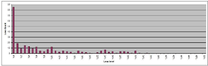
Figure 3.3: DPPI base-case loss distribution conditional on the structure not cashing in

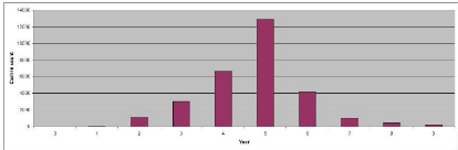
Figure 3.4: Distribution of cash-in times

The Moody's Metric of the base case scenario is 2.697, which is equivalent to an Aa2 rating.

3.4.1 Tailor-made structural features to achieve target rating

Senior rated coupon level

The level of the senior rated coupon is obviously a key parametre in achieving the target rating. The graph below plots the estimated expected loss and Moodys Metric as a function of S, the senior rated premium paid above EURIBOR rate and measured in basis points. One shall point out the jumps in the graph, stemming from the various triggers introduced in the pay-off loss function L. The rather linear relationship outside jumps is also fairly straightforward: between two jumps, the subset of cash-out scenarios is fixed. However, given that the bulk of the loss is explained by scenarios that cash-out at maturity without paying any single coupon, one would find that the average loss on those scenarios is proportional to the senior coupon level, as is the price of a bond paying EURIBOR plus the senior coupon.

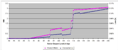
Figure 3.5: Estimated expected loss as a function of S. CDS tenor choices

Initial and reinvestment CDS tenors have a significant impact on the shape of the loss distribution and eventually on its expected level. We now assume that e(.,.) is constant and equal to 0. We then plot the expected loss level as a function of 0 E {3, 4, .., 10}. The reverse-bell shape of the diagram accounts for the fact that:

· for short tenors, the lower MtM volatility of the DPPI does not fully compensate for the loss in contracted CDS spread premia due to the upward sloping shape of the term structure;

· for long tenors, the gain in contracted CDS spread premia does not fully offset the impact of a higher MtM volatility.

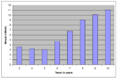
Figure 3.6: Estimated expected loss as a function of è (2000 simulations per coupon level)

Target Notional Exposure parametrization

In order to get the intuition on how the expected loss behaves with respect to the
Target Notional Exposure function TNE(.), one shall slightly simplify the latter and
assume that opportunity leverage and target multiplier functions, OL(.) and TM(.),

are constant and equal to respectively OL and TM. We then plot TNE as a function

of both parametres OL and TM. S1 stands for TM = 20 and S9 for TM = 40 with Si+1 - Si constant.

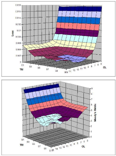
Figure 3.7: Loss and Moody's Metric as a function of OL and TM, 1000 simulations per couple of parametres

One shall point out from the graphs that even with the best combination of fixed

Opportunity Leverage OL and Target Multiplier TM parametres, the structure's
Moody's Metric remains significantly higher than 2.697 obtained with dynamic OL

and TM functions. Also, we clearly see that there is a tradeoff between OL and TM
that allows the structure to improve its rating: too high values for both parametres
lead to a sub-optimal leverage function, reflecting the fact the extra MtM volatility

induced by a higher leverage has a negative fat tail effect on the loss distribution L^(M).

3.4.2 Hypothetical stress-scenarios

Being aware of some obvious limitations in its modelling of risk factors, Moody's requires the DPPI to achieve the target rating in the base-case scenrio and to pass looser target Moody's Metrics in a series of stress-scenarios. Major ones are analyzed hereafter: results are shown in table (3.1).

Credit crisis: systemic brutal spread widening

In order to assess the impact of a brutal widening in CDS spreads, Moody's requires the market spreads of initial long CDS positions to be bumped by á = 25% immediately after the deal's inception. Equivalently, this adverse MtM impact ÄMtM(0) can be expressed in terms of an upfront haircut to be subtracted from the deal's initial notional A:

ÄMtM(0) = á

XN n=1

sn(0)^An(0) A TNE(0) · Dn(0)

where 0 denotes the initial CDS tenor and D_n(0) the initial duration of the n^th CDS. Given initial market conditions and structural features provided in figures (12) and (11), we compute ÄMtM(0) = 3.83% and add this haircut to the initial upfront fee of 1% charged by the arranging investment bank. Results are shown in table (3.1)

Bullish but punctually volatile credit markets: low spreads stressed by punctual default events

The rationale for testing the DPPI in such mixed market environments is to test whether the structure can sustain below-average market spreads, meaning that it does not receive enough CDS premia to cover its liabilities towards investors (the structure is then deemed to be in «negative carry»). To do so, Moody's acts on the parametres of the credit spread process detailed in equation (3.1): it lowers arbitrarily the long term mean â by decreasing ADR as well as b, and divides the volatility parametres ó and ó by two. Results are shown in table (3.1).

Short term default risk concerns: flat credit spread term structure

As seen earlier, the increasing term structure of credit spreads is assumed to be deterministic and to result from a shaping function specific to each rating group. Such an upward slope translates into a positive time-decay when holding long CDS positions. This increasing term structure gets attenuated as ratings get worse: it reflects the fact that conditional on the obligor not defaulting in a near future, its survival probability in the long run is not worse than presently. Moody's cancels that overall positive time-decay effect by assuming a flat credit spread term structure guided by 5-year CDS spread levels. Results are shown in table (3.1).

?n E {1,..,N}, ?t E [0,T], ?0 E [0,10], s_n(t,t + 0) = s_n(t,t + 5)

Hypothetical stress-scenario results

Scenario	L(M)	Moody's Metric		Rating	Base case
0.089%	2.697	Aa2		Early credit crisis
0.248%	4.219	A1		Low spreads
0.447%	5.276	A2		Flat term structure
0.685%	6.091	A3

Table 3.1: DPPI behaviour under base-case and stress scenarios, 20,000 simulations each except for base-case 30,000 draws

As expected, the DPPI's rating worsens in stressed scenarios. The structure's resiliency to adverse market environments is obvious: the magnitude of the potential rating to downgrade is limited to 4 notches in the flat term structure scenario.

3.5 DPPI: any hidden pricing issue?

So far, we have not raised any pricing nor hedging issue pertaining to DPPI products. We shall briefly address both points hereafter.

3.5.1 From the investor's perspective

Initially, the return served to the investor can be split into two separate pieces: the LIBOR/EURIBOR component results from the structure being long a risk-free bond paying an interbank 3-month rate, while the extra risky spread of 100 bps is generated by a long leveraged CDS portfolio. Later on though, the structure may have to realize MtM losses due to a deleveraging signal sent by the portfolio investment rules: in that case, the posted collateral must be partly sold in order to pay for the potential loss on the unwound CDS positions. As a result, the structure is exposed to two major market risks:

· one is the credit risk inherent in holding long CDS positions;

· the other is the interest rate risk created by the potential selling of the collateral before its due term; similarly to what is being done for CSO structures, such a risk is hedged by entering into 3-month forward rate agreements rolled every quarter.

As a result, the DPPI's NPV boils down to being equal to the sum of the par-value of the posted collateral and of the MtM of the long CDS positions. Moreover, from an investor's perspective, it is sensitive only to underlying CDS spread levels and not to interest rates, although the structure's rating will depend on the interest rate curve through its sizing effect on the Reserve R(t).

3.5.2 From the investment bank's perspective

Unlike CSO tranches, which require delta-hedges to be adapted dynamically, DPPI
products do not need any hedging as such. The only market risk that is not passed to
the investor and that is kept within the bank's book is the so-called «gap» risk: in case

of a cash-out event, the bank guarantees the bond floor value to the investor while the structure's NPV may have jumped well below that value due to overnight volatile market conditions. In other words, pricing that initial risk GR(0) (for notation convenience) requires to evaluate quantities such as:

GR(0) = E [(BF(ô) - NPV (ô))¹{ô<ô, NPV (ô)<BF(ô)}B(0,ô)] (3.3)

Given that default processes are pure jump processes, NPV (.) is not continuous either: consequently, GR(0) is not equal to 0. Writing a payoff function such as in equation (3.3) is easy but remains theoretical though: in practise, one would have to assess dependency relationships between interest rate risk factors, which mainly impact the structure's bond floor BF(t), and credit spread levels, which drive the structure's NPV. In other words, pricing each payoff component of the DPPI is a challenging task that can only be addressed in simplified frameworks such as the one described in [25] (time-continuous processes with discrete trading dates).

Another way of evaluating that gap risk is to look at the potential MtM impact of names defaulting in the portfolio when the NPV gets close to the Bond Floor BF: by construction, the function TM(t)R(t) has a mitigating impact on that risk: as the Reserve R(t) shrinks, TM(t)R(t) starts driving down the Target Notional Exposure TNE(t), hence reducing the MtM impact of any potential default. More generally, assuming all N names in portfolio are equally weighted with identical deterministic recovery rates RR and that readjustment bounds l_u and ld are set to 0, we can express the MtM impact of one default ÄMtM(1) as:

1 - RR

ÄMtM(1) = N · TNE(t)

We then want to give a lower bound for ND(t) defined as the number of defaults the structure can sustain before its reserve R(t) is fully wiped out:

R(t)

?t ? [0,T], ND(t) : = ÄMtM(1)

R(t)
TNE(t)

N

= 1-RR ·

= N 1 - RR ·	1
	TM(t)

= N

1 - RR(DR + SR(t) · D(t))

N

= 1-RR · DR

This last term does not depend on t. Assuming RR = 40%, N = 135 and DR = 1%, we find that ?t ? [0, T], ND(t) = 2.25. In other words, at any point in time, the structure can stand 2 simultaneous defaults before breaking the bond floor in the worst case scenario.

Conclusion

In this document, we have presented a theoretical modelling framework for designing and rating a Dynamic Proportion Portfolio Insurance (DPPI)) product, an innovation in the world of synthetic structured credits providing a capital guarantee to the investor.

We first outline the main steps of Collateral Synthetic Obligation risk-neutral pricing in the well-known one factor gaussian copula model, which we further develop and supplement for rating DPPIs. However, the latter requires to evaluate an expected loss function L^(M) under the historical risk measure: various discrete and continuous random processes are introduced for describing risk factors such as defaults, rating transitions, Credit Default Swap (CDS) spread levels and recovery rates. Process parametres calibrated on historical data are assumed to be provided by Moody's, a rating agency. We then rely upon a C++ implementation to run Monte-Carlo simulations and estimate L^(M).

The combination of several innovative investment rules such as a dynamic leverage function, contingent coupon payments, the removal of downgraded assets, lock-in and lock-out features, allows us to minimize L^(M), achieve the target rating of Aa3 in the base case scenario and pass all required stress scenarios.

Finally, we describe the «gap-risk» hedging issue faced by the investment bank when granting a capital guarantee to the investor. We show that in a simplified framework, it can be measured through a default-count equivalent function closely related to the DPPI's structural features.

Appendix

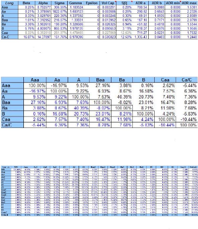
Figure 8: Parametres of Moody's CDS spread processes

Figure 9: Correlation matrix of Moody's CDS spread processes

Figure 10: Moody's 10Y corporate rating transition matrix

Moody's risk factors

Optimized DPPI parametres

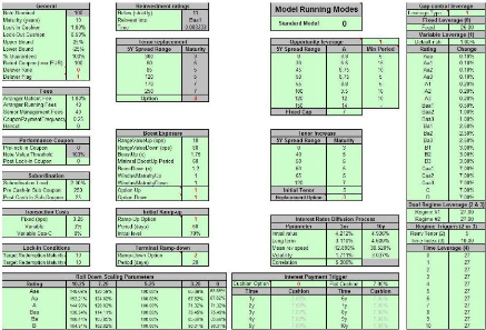
Figure 11: DPPI optimized structural features

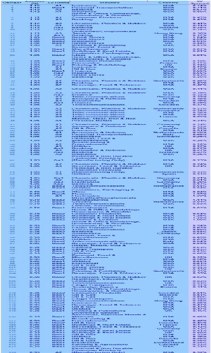
Figure 12: DPPI reference portfolio
41

Bibliography

[1] L. ANDERSEN, J. SIDENIUS & S. BASU, All your hedges in one basket, RISK magazine, 2003

[2] J-P. LAURENT, J. GREGORY, Basket default swaps, CDOs and factor copulas, Working paper, 2003

[3] D.X. LI, On default correlation: a copula factor approach, The Journal of Fixed Income, 2000

[4] A. ELIZALDE, Credit Risk Models IV: understanding and pricing CDOs, Working paper No. 0608, CEMFI, 2006

[5] Q. CHEN, CDO Pricing and Copula Method, Working paper, University of Maryland, 2006

[6] A. LÜSCHER, Synthetic CDO pricing using the double normal inverse Gaussian copula with stochastic factor loadings, Master's thesis, ETH Zürich, 2005

[7] B. VERSCHUERE, On copulas and their application to CDO pricing, Master's thesis, University Of Toronto, 2006

[8] M. VAN DER VOORT, Factor copulas: totally external defaults, Working paper, ABN Amro, 2005

[9] E. PARCELL, Loss unit interpolation in the collateralized debt obligation pricing model, Working paper, Derivative Fitch, 2006

[10] S. GALIANI, M. SHCHETKOVSKIY & A. KAKODKAR, Factor models for synthetic CDO valuation, Internal working paper, Merrill Lynch, 2004

[11] M. SHCHETKOVSKIY et al, Base correlation and beyond, Internal working paper, Merrill Lynch, 2006

[12] A. PAIN, O. RENAULT & D. SHELTON, Base correlation: the term structure dimension, Internal working paper, Citigroup, 2005

[13] P. TEKLOS et al, CPDOs: the new best seller?, Special report, Citigroup, 2006

[14] E. VARLOOT, CPDO: an asset class of its own or a glorified bearish rated equity?, Special report, Union des Banques Suisses, 2006

[15] A. LINDEN et al, First Generation CPDO: case study on performance and ratings, Special report, Derivative Fitch, 2007

[16] B. MARJOLIN et al, Moody's approach to modelling Exotic synthetic CDOs with CDOROM, Special report, Moody's, 2007

[17] A. KAROLIK, Modeling Correlated Credit Rating Migrations, PhD thesis, Carnegie Mellon University, 2006

[18] D. BUNIMOVICH, Modeling and Pricing of Collateralized Debt Obligations, PhD thesis, Carnegie Mellon University, 2002

[19] V. DURRLEMANN, Les fonctions copules: définition, examples et propriétés, Class notes, Ecole Nationale des Ponts et Chaussées, 2006

[20] J-F. DELMAS, Mesures de risque, Class notes, Ecole Nationale des Ponts et Chaussées, 2006

[21] P. MAZAUTAUD et al, Moody's Metric and Its Uses, Special report, Moody's, 2006

[22] A. METZ, R. CANTOR, Introducing Moody's Credit Transition Model, Special report, Moody's 2007

[23] A. METZ, R. CANTOR, A Cyclical Model of Multiple-Horizon Credit Rating Transitions and Default, Special report, Moody's, 2007

[24] A. GUTTLER, Conditional Rating Transitions: The Case of S&P and Moody's, European Business School, Working paper, 2007

[25] S. BALDER, M. BRANDL & A. MAHAYNI, Effectiveness of CPPI Strategies under Discrete-Time Trading, University of Bonn, Working paper, 2005