b) Afficher les quatre séquences
numériques


10 20 30


1 0.8 0.6 0.4 0.2
0
1 0.8 0.6 0.4 0.2
0
2 4 6
|
1 0.8 0.6
|
|
|
|
|
|
1
0.5
0
-0.5
-1
|
|
|
|
|
|
|
|
|
|
0.4
0.2
0
|
|
|
|
|
|
|
|
|
0 20 40 60
0 20 40 60
- 18 -
III Partie Travail Pratique N3 : Conversion
de modèles
Conversion d'un model état à un model de
la fonction de transfert
Code :
sys_tf=tf(1.5, [1 9 30.6])
ésultat:
Transfer function: 1.5
s^2 + 9 s + 30.6
conversion en modele zpk
code
sys_zpk=zpk([0, -2], [4, 3.6], 9)
ésultat:
Zero/pole/gain: 9 s (s+2)
(s-4) (s-3.6)
Affichage des paramètres
Code:
a=3; b=7; c=1; d=11;
sys=ss(a,b,c,d)
Résultat:
a =
x1
x1 3
b=
u1
x1 7
c =
x1
y1 1
d=
u1
y1 11
Continuous-time model.
- 20 -
Simulation d'un modèle d'espace
Considérons le système LTI ci-dessous :
UL UR
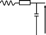

i1
UC
U1
i2
i3
U2
1) X(I,U) ; dX /dt = AX + B A et B étant des matrices.
2) Y= CX+D C et D étant des matrices.
Donnons des valeurs à nos matrices.
Etude
Apres étude de ce système on obtient l'expression
suivante
En posant X= (i1 ;u2)
. dX= (R/L 1/L ; 1/C 0) * X + (-1/L ; 0) U1.
Par correspondance avec l'expression .dX= Ax +BU1
On obtient et les matrices suivantes A= (R/L 1/L ; 1/C 0)
B= (-1/L ; 0)
Par ailleurs, U2=U2 donc,
U2= (0 ; 1) (i1 ; U2)
Par correspondance avec l'expression
U2= CX + D On Obtient C= (0 ; 1)
D= (0)
Choisissons R=5 ohms L= 10H
C=50mF
Donc
A= (0.5 0.1 ; 20 0)
B= (-0.1 ; 0) C= (0 ; 1)
D= (0)
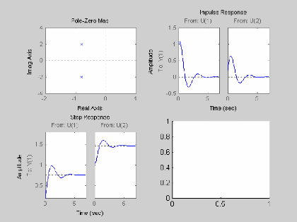
Simuler un modèle d'espace de mon choix
Soit les matrices a, b, c et d
Code:
a=[-.8 2 ;-2 -.8];
b=[1 .2;.9 1];
c=[1 0];
d=[.2 1];
subplot(2,2,1); pzmap(a,b,c,d)
subplot(2,2,2); impulse(a,b,c,d)
subplot(2,2,3); step(a,b,c,d)
subplot(2,2,4); initial(a,b,c,d)
ésultat:
|