Memoire Online - An Assessment of plankton diversity as an water quality indicator in small man-made reservoirs in the Mzingwane catchment, Limpopo basin, Zimbabwe

The study sites exhibited seasonal variation in the abundance of phytoplankton and zooplankton (Fig 3.7 and Fig. 3.8). The highest abundance of zooplankton was recorded in February while the highest abundance of phytoplankton was recorded in April.

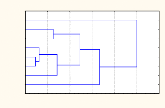
A clustering of stations according to plankton abundance using complete linkage is presented in Fig 3.9 and Fig.3.10. These figures show Sibasa and Mpopoma reservoirs' abundance being very dissimilar to all other reservoirs in February while Sibasa, Makoshe and Mezilume are very dissimilar to others in April. No similarity is found between reservoirs according to their presence or not in the National Park or in the communal lands. A first level similarity is found in February between Chitampa (National Park), Makoshe and Dewa (Communal Lands) similarity in abundance of stations according to their occurrence in the National Park or in the communal lands is depicted. However, these Figures show how close the studied reservoirs were in terms of abundance. Different linkages between the two sampling periods can be found as well when comparing these clusters.

Fig. 3.9 Clustering of stations according to the overall plankton abundance/ February

Fig. 3.10 Clustering of stations according to the overall plankton abundance/ April

3.1.4 Relationships between physico-chemical parameters and plankton species in the studied reservoirs

A comparison of the National Park and communal lands for a number of parameters and species relationships showed significant differences (annexes 5 and 6). The following elements showed a significant difference taking Mezilume (National Park) and Makoshe (Communal lands) as an example: pH of water (P<0.01), electroconductivity of water (P<0.001), total nitrogen (P <0.05), the cladoceran Moina (P <0.05), the cyanophyte Anabaena (P <0.05), and the dinophyte Ceratium (P <0.05).

The colour of water may have had an influence on the following elements using ANOVA: pH of water (P<0.01), electroconductivity of water (P<0.001), total nitrogen (P<0.0 1), hardness of water (P<0.0 1), soil' s electroconductivity (P<0.0 1), the species Daphnia (P<0.001), Brachionus (P<0.01), Microdides (P <0.05), nauplii cyclopoids (P <0.05), nauplii calanoids (P <0.05), Anabaena (P<0.01), Peridinium (P<0.001), Melosira (P <0.05), Scenedesmus (P <0.05), Pediastrum (P<0.01), Hydrodictyon (P<0.01), Dinobryon (P <0.05), Pleurotaenium (P<0.01), Arthrodesmus (P <0.05), Fragilaria (P <0.05) and Zygnema (P <0.05). The soil type also showed a significant influence on some phytoplankton species.

The clustering of all the components of the main biota in relation to the water quality is presented on Fig. 3.11 and 3.12. These figures highlight the relationships of species found in the study area with its chemistry. Total phosphorus, total nitrogen in the small reservoirs and electroconductivity of soils had a relationship with zooplankton (Daphnia, Rotifera, Brachionus and Ostracoda) and phytoplankton taxa (Navicula, Phacus, Lepadella, Sphaerocystis, Staurodesmus, Cosmarium and Sporangium). The pH of water and soils, water hardness and electroconductivity also influenced some species (Fig. 3.11 and 3.12).

Factor Loadings, Factor 1 vs. Factor 2
Rotation: Unrotated
Extraction: Principal axis factoring

Fig. 3.11 Relationship between chemistry and zooplankton in the studied reservoirs

Taxa abbreviations: Nauplii cyclopoids (NAUPLCYC), Nauplii calanoids (NAUPLCA), Microdides (MICRODID), Cladocera (CLADOCER),

Abiotic elements abbreviations: Total Nitrogen (TNWATER), Total Phosphorus in water (TPWATER), electroconductivity in soils (ECSOIL), water hardness (HARDWAT), water' s electroconductivity (ECWAT)

Factor Loadings, Factor 1 vs. Factor 2
Rotation: Unrotated
Extraction: Principal axis factoring

	0.6 0.4 0.2 0.0 -0.2 -0.4 -0.6 -0.8 -1.0 -1.2
			STAURODE
			NAVICULA COSMARIU
MELOSIRA			PHACUS TPWATER	RHIZOSOL
ECWAT			LEPADELL TNWATER
ANABAENA
HARDNWAT		GYROSIGM		ECSOIL
PHWATER
			SPHAEROC
PH, hardness and EC			SPORANGI TN and TP
PHSOIL
			CLOSTERI
			SYNEDRA
			PERIDINI EUGLENA
			CERATIUM

Fig. 3.12 Relationship between chemistry and phytoplankton in the studied reservoirs.

Taxa abbreviations: Gyrosigma (GYROSIGM), Lepadella (LEPADELL), Staurodesmus (STAURODE), Cosmarium (COSMARIO), Rhizosolenia (RHIZOSOL), Sphaerocystis (SPHAEROC), Sporangium (SPORANGI), Closterium (CLOSTERI).

Abiotic elements abbreviations: Total Nitrogen (TNWATER), Total Phosphorus in water (TPWATER), electroconductivity in soils (ECSOIL), water hardness (HARDWAT), water' s electroconductivity (ECWAT)

An Assessment of plankton diversity as an water quality indicator in small man-made reservoirs in the Mzingwane catchment, Limpopo basin, Zimbabwe

3.1.3 Overall plankton abundance

3.1.4 Relationships between physico-chemical parameters and plankton species in the studied reservoirs